MBO Sparse Maps

This tutorial illustrates how using elastic costs of the form

\[ c(x, y) = h_\tau(x - y)\text{ with } h_\tau(z) = \frac12\|z\|^2_2 + \tau(z), \]

when estimating Monge maps that are optimal for that cost results in displacement that have structure. In full generality \(\tau\) can be any regularizer that has a proximal operator known in closed form. We will consider in particular the \(\ell_1\) sparsity-inducing norm.

Entropic Monge maps estimated from samples using such a cost exhibit sparsity in displacements: every input point is transported to another target point by only changing a subset of its features.

import sys

if "google.colab" in sys.modules:
    !pip install -q git+https://github.com/ott-jax/ott@main

  Installing build dependencies ... ?25l?25hdone
  Getting requirements to build wheel ... ?25l?25hdone
  Installing backend dependencies ... ?25l?25hdone
  Preparing metadata (pyproject.toml) ... ?25l?25hdone

import jax
import jax.numpy as jnp

import matplotlib.pyplot as plt

import ott
from ott.geometry import costs, pointcloud
from ott.problems.linear import linear_problem
from ott.solvers.linear import sinkhorn

Sampling 2D point clouds

n_source = 30
n_target = 50
n_test = 10
p = 2

key = jax.random.PRNGKey(0)
keys = jax.random.split(key, 4)
x = jax.random.normal(keys[0], (n_source, p))

y0 = jax.random.normal(keys[1], (n_target // 2, p)) + jnp.array([5, 0])
y1 = jax.random.normal(keys[2], (n_target // 2, p)) + jnp.array([0, 8])
y = jnp.concatenate([y0, y1])

# Plotting utility
def plot_map(x, y, x_new=None, z=None, ax=None, title=None):
    if ax is None:
        f, ax = plt.subplots(figsize=(10, 8))

    ax.scatter(*x.T, s=200, edgecolors="k", marker="o", label=r"$x$")
    ax.scatter(*y.T, s=200, edgecolors="k", marker="X", label=r"$y$")
    if z is not None:
        ax.quiver(
            *x_new.T,
            *(z - x_new).T,
            color="k",
            angles="xy",
            scale_units="xy",
            scale=1,
            width=0.007,
        )
        ax.scatter(
            *x_new.T, s=150, edgecolors="k", marker="o", label="$x_{new}$"
        )
        ax.scatter(
            *z.T,
            s=150,
            edgecolors="k",
            marker="X",
            label=r"$T_{x\rightarrow y}(x_{new})$",
        )
    if title is not None:
        ax.set_title(title)
    ax.legend(fontsize=22)

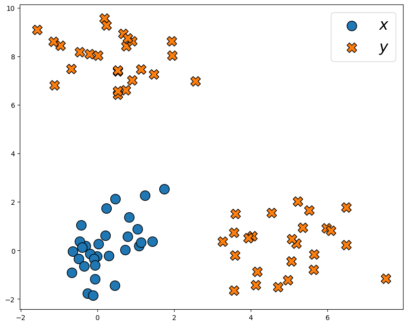
The source samples \(x\) are drawn from a Gaussian distribution, while the target samples \(y\) are drawn from a mixture of two Gaussians.

plot_map(x, y)

We also draw some fresh unseen samples from the source distribution:

n_new = 10
x_new = jax.random.normal(keys[3], (n_new, p))

Standard entropic Monge map

We first compute the “standard” entropic map between these two distributions using the \(\ell_2^2\) cost. Following [Pooladian and Niles-Weed, 2021], we compute the solution of Sinkhorn on the problem, and then use OTT to turn these solutions into a pair of dual potentials functions.

These dual potentials are then used to build the entropic map with the transport() method.

# jit first a Sinkhorn solver.
solver = jax.jit(sinkhorn.Sinkhorn())


def entropic_map(x, y, cost_fn: costs.TICost) -> jnp.ndarray:
    geom = pointcloud.PointCloud(x, y, cost_fn=cost_fn)
    output = solver(linear_problem.LinearProblem(geom))
    dual_potentials = output.to_dual_potentials()
    return dual_potentials.transport


map = entropic_map(x, y, costs.SqEuclidean())

plot_map(x, y, x_new, map(x_new))

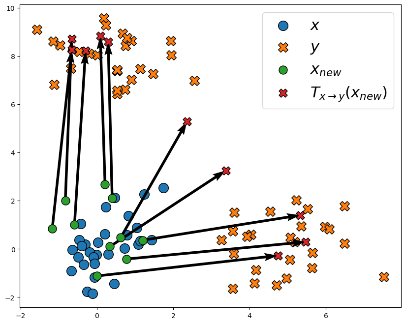
We see that the displacements have no particular structure.

Sparse Monge displacements

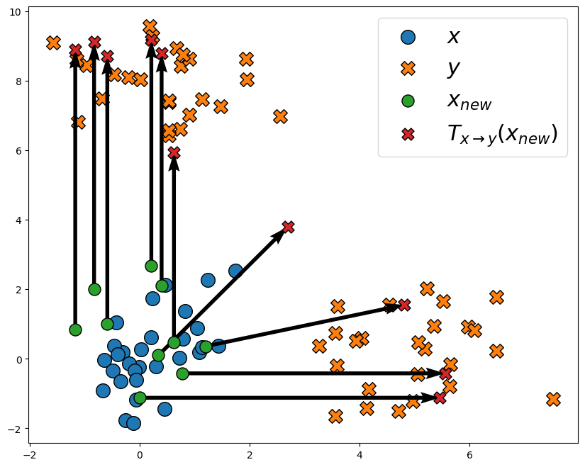
We now turn to mixed costs, with the ElasticL1 cost that corresponds to the function

\[ h(z) = \frac12\|z\|_2^2 + \text{scaling_reg} \|z\|_1. \]

map_l1 = entropic_map(x, y, costs.ElasticL1(scaling_reg=10.0))

plot_map(x, y, x_new, map_l1(x_new))

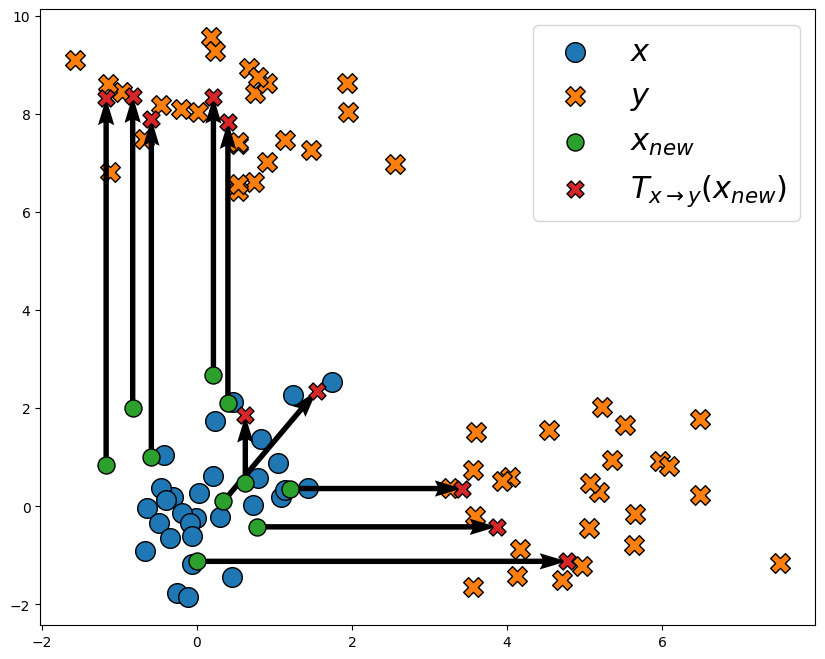
We now see that most samples have a sparse displacement patterns: for most samples, only one coordinate is changed. In this case, that coordinate depends on the sample: some samples move only along the x-axis, while other move only along the y-axis. Some points also move along both axes.

We can investigate the effect of the regularization strength scaling_reg on the estimated maps:

scaling_regs = [0.1, 1.0, 10.0, 100.0]

f, axe = plt.subplots(2, 2, figsize=(15, 12))
for scaling_reg, ax in zip(scaling_regs, axe.ravel()):
    map = entropic_map(x, y, costs.ElasticL1(scaling_reg=scaling_reg))
    plot_map(
        x,
        y,
        x_new,
        map(x_new),
        ax=ax,
        title=rf"$scaling\_reg = {scaling_reg}$",
    )

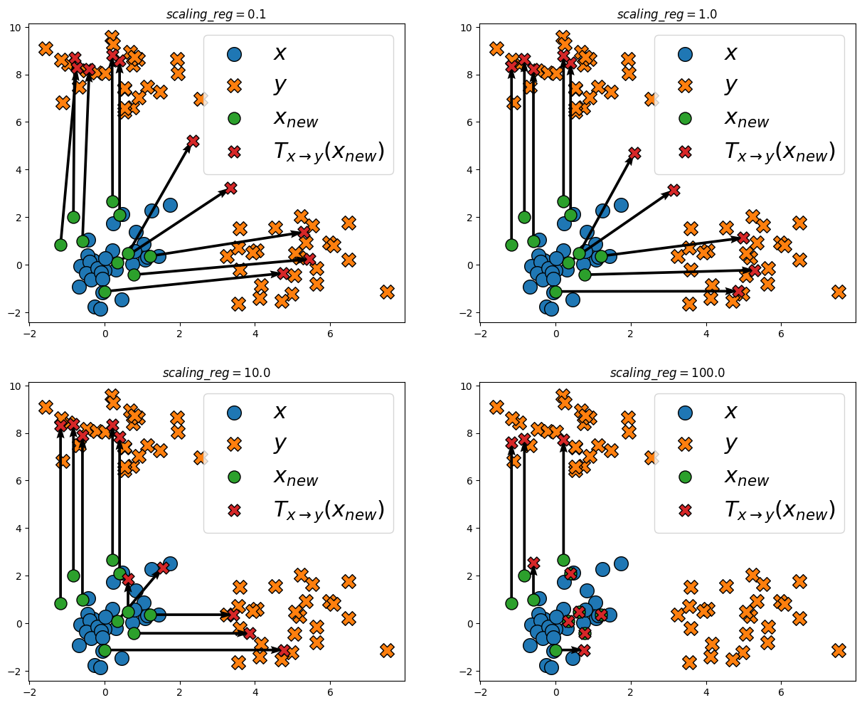
We see that a low scaling_reg leads to no sparsity in the displacements. Increasing scaling_reg, sparsity starts appearing. Taking a really high scaling_reg also leads to a large shrinkage, as evident in the last plot.

We can also consider other sparsity inducing norms like the \(k\)-overlap [Argyriou et al., 2012] :

\[ h(z) = \frac12\|z\|_2^2+\text{scaling_reg}\|z\|_{k-ov} \]

map = entropic_map(x, y, costs.ElasticSqKOverlap(k=1, scaling_reg=1.0))

plot_map(x, y, x_new, map(x_new))

This cost induces less shrinkage, but requires more computational effort than the simple soft-thresholding operator.