Low-rank Sinkhorn

We experiment with the low-rank LRSinkhorn solver, proposed by [Scetbon et al., 2021] as an alternative to the Sinkhorn algorithm.

The idea of that solver is to compute optimal transport couplings that are low-rank, by design. Rather than look for a \(n\times m\) matrix \(P_\varepsilon\) that has a factorization \(D(u)\exp(-C/\varepsilon)D(v)\) (as computed by the Sinkhorn algorithm) when solving a problem with cost \(C\), the set of feasible plans is restricted to those adopting a factorization of the form \(P_r = Q D(1/g) R^T\), where \(Q\) is \(n\times r\), \(R\) is \(r \times m\) are two thin matrices, and \(g\) is a \(r\)-dimensional probability vector.

import sys

if "google.colab" in sys.modules:
    !pip install -q git+https://github.com/ott-jax/ott@main

import jax
import jax.numpy as jnp

import matplotlib.pyplot as plt

from ott.geometry import pointcloud
from ott.problems.linear import linear_problem
from ott.solvers.linear import sinkhorn, sinkhorn_lr
from ott.tools import plot

def create_points(rng, n, m, d):
    rngs = jax.random.split(rng, 4)
    x = jax.random.normal(rngs[0], (n, d)) + 1
    y = jax.random.uniform(rngs[1], (m, d))
    a = jax.random.uniform(rngs[2], (n,))
    b = jax.random.uniform(rngs[3], (m,))
    a = a / jnp.sum(a)
    b = b / jnp.sum(b)
    return x, y, a, b

Create a LinearProblem comparing two point clouds.

rng = jax.random.PRNGKey(0)
n, m, d = 19, 35, 2
x, y, a, b = create_points(rng, n=n, m=m, d=d)

geom = pointcloud.PointCloud(x, y, epsilon=0.1)
ot_prob = linear_problem.LinearProblem(geom, a, b)

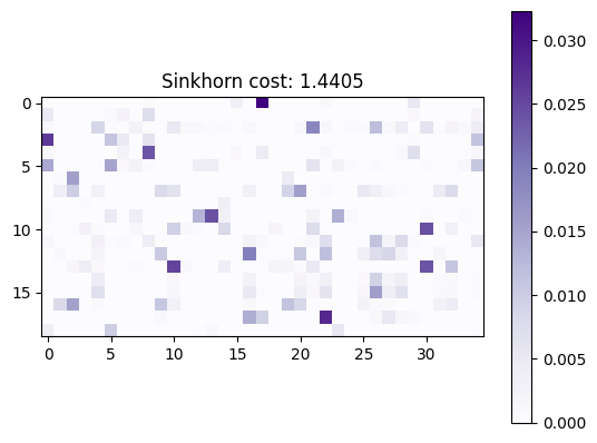
Solve linear OT problem with Sinkhorn

solver = sinkhorn.Sinkhorn()
ot_sink = solver(ot_prob)

plt.imshow(ot_sink.matrix, cmap="Purples")
plt.title(f"Sinkhorn cost: {ot_sink.primal_cost:.4f}")
plt.colorbar()
plt.show()
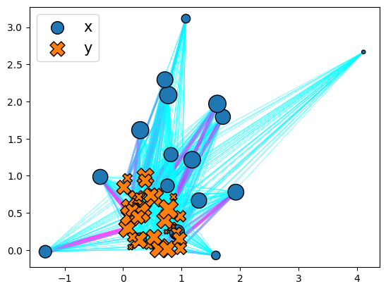
plott = plot.Plot()
_ = plott(ot_sink)

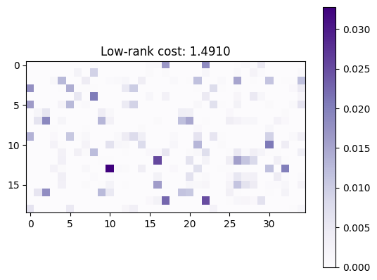
Solve linear OT problem with low-rank Sinkhorn

Solve the problem using the LRSinkhorn solver, with a rank parameterized to be equal to the half of \(r=\min(n,m)/2\)

solver = sinkhorn_lr.LRSinkhorn(rank=int(min(n, m) / 2))
ot_lr = solver(ot_prob)

transp_cost = ot_lr.compute_reg_ot_cost(ot_prob)
plt.imshow(ot_lr.matrix, cmap="Purples")
plt.colorbar()
plt.title(f"Low-rank cost: {ot_lr.primal_cost:.4f}")
plt.show()
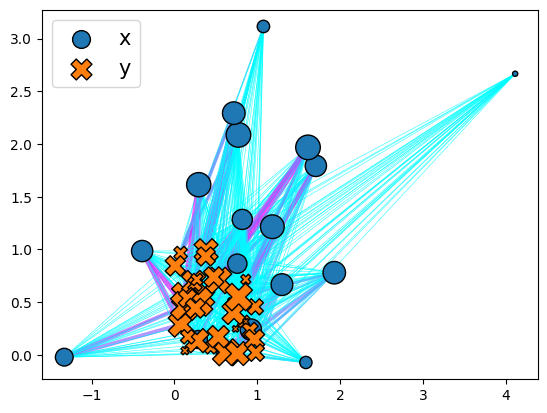
plott = plot.Plot()
_ = plott(ot_lr)

Play with larger scales

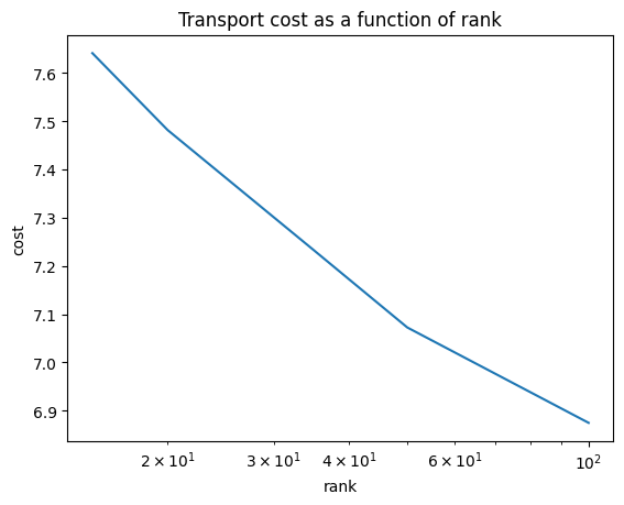
One of the interesting features of the low-rank approach lies in its ability to scale, since its iterations are of complexity \(O( (n+m) r)\) rather than \(O(nm)\). We consider this by sampling two points clouds of size \(n=m=100\ 000\) in \(d=7\).

n, m, d = 10**5, 10**5 + 1, 7
x, y, a, b = create_points(rng, n=n, m=m, d=d)

We compute plans that satisfy a rank constraint \(r\), for various values of \(r\).

geom = pointcloud.PointCloud(x, y, epsilon=0.1)
ot_prob = linear_problem.LinearProblem(geom, a, b)
costs = []
ranks = [15, 20, 35, 50, 100]
for rank in ranks:
    solver = jax.jit(sinkhorn_lr.LRSinkhorn(rank=rank, initializer="k-means"))
    ot_lr = solver(ot_prob)
    costs.append(ot_lr.reg_ot_cost)

As expected, the optimal cost decreases with rank, as shown in the plot below. Recall that, because of the non-convexity of the original problem, there may be small bumps along the way.

For these two fairly concentrated distributions, it seems possible to produce plans that have relatively small rank yet low cost.

plt.plot(ranks, costs)
plt.xscale("log")
plt.xlabel("rank")
plt.ylabel("cost")
plt.title("Transport cost as a function of rank")
plt.show()