%load_ext autoreload
%autoreload 2

Gromov-Wasserstein

In this tutorial, we present the GromovWasserstein [Mémoli, 2011] solver. The goal of the GW problem is to match two point clouds, taken from different spaces endowed with their own geometries. We illustrate this use case by aligning a 2-d to a 3-d point clouds, see also GW for Multi-omics for a more challenging application to single-cell omics.

import sys

if "google.colab" in sys.modules:
    !pip install -q git+https://github.com/ott-jax/ott@main

import jax
import jax.numpy as jnp
import numpy as np

import matplotlib.pyplot as plt
import mpl_toolkits.mplot3d.axes3d as p3
from IPython import display
from matplotlib import animation, cm

from ott.geometry import pointcloud
from ott.problems.quadratic import quadratic_problem
from ott.solvers.quadratic import gromov_wasserstein

Matching across spaces

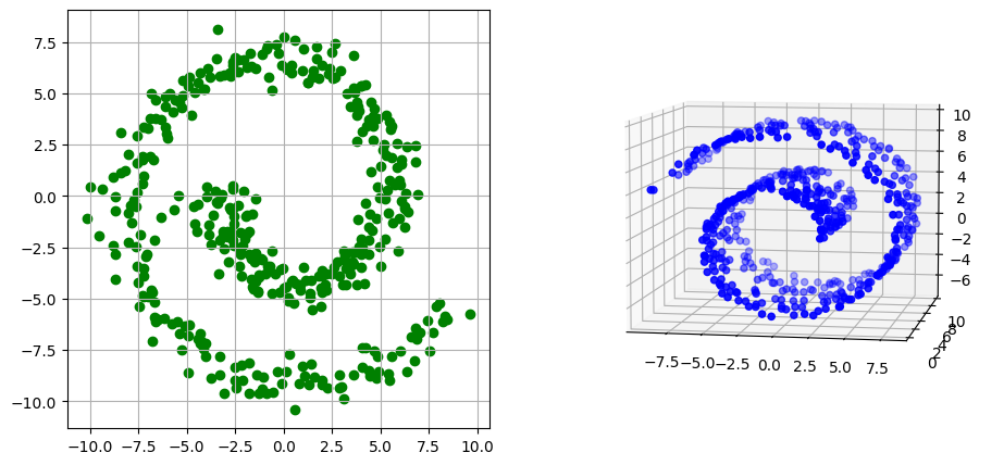
We use the GromovWasserstein solver to match a spiral in 2-d to a Swiss roll in 3-d, generated below

def sample_spiral(
    n, min_radius, max_radius, key, min_angle=0, max_angle=10, noise=1.0
):
    radius = jnp.linspace(min_radius, max_radius, n)
    angles = jnp.linspace(min_angle, max_angle, n)
    data = []
    noise = jax.random.normal(key, (2, n)) * noise
    for i in range(n):
        x = (radius[i] + noise[0, i]) * jnp.cos(angles[i])
        y = (radius[i] + noise[1, i]) * jnp.sin(angles[i])
        data.append([x, y])
    data = jnp.array(data)
    return data


def sample_swiss_roll(
    n, min_radius, max_radius, length, key, min_angle=0, max_angle=10, noise=0.1
):
    spiral = sample_spiral(
        n, min_radius, max_radius, key[0], min_angle, max_angle, noise
    )
    third_axis = jax.random.uniform(key[1], (n, 1)) * length
    swiss_roll = jnp.hstack((spiral[:, 0:1], third_axis, spiral[:, 1:]))
    return swiss_roll


def plot(
    swiss_roll, spiral, colormap_angles_swiss_roll, colormap_angles_spiral
):
    fig = plt.figure(figsize=(11, 5))
    ax = fig.add_subplot(1, 2, 1)
    ax.scatter(spiral[:, 0], spiral[:, 1], c=colormap_angles_spiral)
    ax.grid()
    ax = fig.add_subplot(1, 2, 2, projection="3d")
    ax.view_init(7, -80)
    ax.scatter(
        swiss_roll[:, 0],
        swiss_roll[:, 1],
        swiss_roll[:, 2],
        c=colormap_angles_swiss_roll,
    )
    ax.set_adjustable("box")
    plt.show()

# Generation parameters
n_spiral = 400
n_swiss_roll = 500
length = 10
min_radius = 3
max_radius = 10
noise = 0.8
min_angle = 0
max_angle = 9
angle_shift = 3

# Seed
rng = jax.random.PRNGKey(14)
rng, *subrngs = jax.random.split(rng, 4)

spiral = sample_spiral(
    n_spiral,
    min_radius,
    max_radius,
    key=subrngs[0],
    min_angle=min_angle + angle_shift,
    max_angle=max_angle + angle_shift,
    noise=noise,
)
swiss_roll = sample_swiss_roll(
    n_swiss_roll,
    min_radius,
    max_radius,
    key=subrngs[1:],
    length=length,
    min_angle=min_angle,
    max_angle=max_angle,
)

plot(swiss_roll, spiral, "blue", "green")

We define two point clouds to describe each of these point clouds, each using (by default) the SqEuclidean cost function.

# Instantiate the Quadratic Alignment Problem
geom_xx = pointcloud.PointCloud(x=spiral, y=spiral)
geom_yy = pointcloud.PointCloud(x=swiss_roll, y=swiss_roll)
prob = quadratic_problem.QuadraticProblem(geom_xx, geom_yy)

# Instantiate a jitt'ed Gromov-Wasserstein solver
solver = jax.jit(
    gromov_wasserstein.GromovWasserstein(
        epsilon=100.0, max_iterations=20, store_inner_errors=True
    )
)
out = solver(prob)

has_converged = bool(out.linear_convergence[out.n_iters - 1])
print(f"{out.n_iters} outer iterations were needed.")
print(f"The last Sinkhorn iteration has converged: {has_converged}")
print(f"The outer loop of Gromov Wasserstein has converged: {out.converged}")
print(f"The final regularized GW cost is: {out.reg_gw_cost:.3f}")

5 outer iterations were needed.
The last Sinkhorn iteration has converged: True
The outer loop of Gromov Wasserstein has converged: True
The final regularized GW cost is: 1183.611

The resulting transport matrix between the two point clouds is as follows:

transport = out.matrix
fig = plt.figure(figsize=(8, 6))
plt.imshow(transport, cmap="Purples")
plt.xlabel(
    "IDs of samples from the Swiss roll", fontsize=14
)  # IDs are ordered from center to outer part
plt.ylabel(
    "ID of samples from the spiral", fontsize=14
)  # IDs are ordered from center to outer part
plt.colorbar()
plt.show()

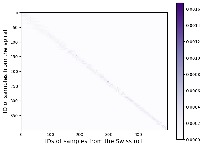
The larger the regularization parameter epsilon is, the more diffuse the transport matrix becomes, as we can see in the animation below.

# Animates the transport matrix
fig = plt.figure(figsize=(8, 6))
im = plt.imshow(transport, cmap="Purples")
plt.xlabel(
    "IDs of samples from the Swiss roll", fontsize=14
)  # IDs are ordered from center to outer part
plt.ylabel(
    "IDs of samples from the spiral", fontsize=14
)  # IDs are ordered from center to outer part
plt.colorbar()


# Initialization function
def init():
    im.set_data(np.zeros(transport.shape))
    return [im]


# Animation function
def animate(i):
    array = im.get_array()
    geom_xx = pointcloud.PointCloud(x=spiral, y=spiral)
    geom_yy = pointcloud.PointCloud(x=swiss_roll, y=swiss_roll)
    prob = quadratic_problem.QuadraticProblem(geom_xx, geom_yy)

    solver = gromov_wasserstein.GromovWasserstein(epsilon=i, max_iterations=20)

    out = solver(prob)

    im.set_array(out.matrix)
    im.set_clim(0, jnp.max(out.matrix[:]))
    return [im]


# Call the animator
anim = animation.FuncAnimation(
    fig,
    animate,
    init_func=init,
    frames=[70.0, 100.0, 200.0, 500.0, 750.0, 1000.0, 2000.0, 10000.0, 50000.0],
    interval=1500,
    blit=True,
)

html = display.HTML(anim.to_jshtml())
display.display(html)
plt.close()

Once Loop Reflect

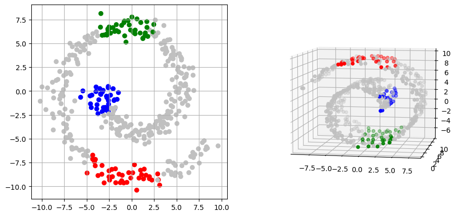
To better understand the correspondence found by the GromovWasserstein solver, we plot in the same color, for each point in the spiral, the point in the Swiss roll it is the most coupled to.

# For each sample from the spiral, we get the most coupled point from the Swiss roll
indices_swiss_roll = jnp.array(np.argmax(transport, axis=1))

# Sets colors to visualise matching of some areas between each shape
# IDs of spiral and Swiss roll are ordered from center to outer part
colors_input_spiral = (
    ["b"] * 40
    + ["silver"] * 160
    + ["g"] * 40
    + ["silver"] * 90
    + ["r"] * 40
    + ["silver"] * 30
)
colors_swiss_roll = np.array(["silver"] * 500)
colors_swiss_roll[indices_swiss_roll[:40]] = "b"
colors_swiss_roll[indices_swiss_roll[200:240]] = "g"
colors_swiss_roll[indices_swiss_roll[330:370]] = "r"

plot(swiss_roll, spiral, colors_swiss_roll, colors_input_spiral)