
Getting Started#
This short tutorial covers a basic use case for ott:
Compute an optimal transport between two point clouds. This solves a problem that is described by a
PointCloudgeometry object (to describe pairwise distances between the points), which is then fed in theSinkhornalgorithm.Showcase the seamless integration with
jax, to differentiate through that OT distance, and plot the gradient flow of that distance, to morph the first point cloud into the second.
Imports and toy data definition#
import sys

if "google.colab" in sys.modules:
    %pip install -q git+https://github.com/ott-jax/ott@main
import jax
import jax.numpy as jnp

import matplotlib.pyplot as plt

from ott.geometry import pointcloud
from ott.solvers import linear
ott is built on top of jax, so we use jax to instantiate all variables. We generate two 2-dimensional random point clouds of \(7\) and \(11\) points, respectively, and store them in variables x and y:
rngs = jax.random.split(jax.random.PRNGKey(0), 2)
d, n_x, n_y = 2, 7, 11
x = jax.random.normal(rngs[0], (n_x, d))
y = jax.random.normal(rngs[1], (n_y, d)) + 0.5
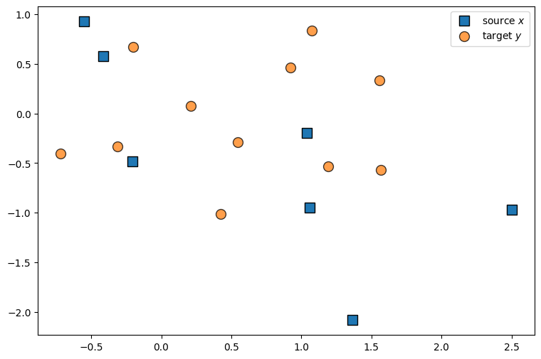
Because these point clouds are 2-dimensional, we can use scatter plots to illustrate them.
x_args = {"s": 100, "label": r"source $x$", "marker": "s", "edgecolor": "k"}
y_args = {"s": 100, "label": r"target $y$", "edgecolor": "k", "alpha": 0.75}
plt.figure(figsize=(9, 6))
plt.scatter(x[:, 0], x[:, 1], **x_args)
plt.scatter(y[:, 0], y[:, 1], **y_args)
plt.legend()
plt.show()
Optimal transport with ott#
We will now use ott to compute the optimal transport between x and y. To do so, we first create a geom object that stores the geometry (a.k.a. the ground cost) between x and y:
geom = pointcloud.PointCloud(x, y, cost_fn=None)
geom holds the two datasets x and y, as well as a cost_fn, a function used to quantify a cost between two points. Here, we passed no cost_fn; this defaults to cost_fn equal to SqEuclidean, the usual squared-Euclidean distance between two points, \(c(x,y)=\|x-y\|^2_2\).
In order to compute the optimal coupling corresponding to geom, we use the Sinkhorn algorithm, wrapped in the convenience wrapper solve(). The Sinkhorn algorithm will use a regularization hyperparameter epsilon, which is typically of the scale of \(c(x,y)\) found across point-clouds. For this reason, ott stores that parameter in geom, and uses by default the twentieth of the mean cost between all points in x and y. While it is also possible to set probably weights a for each point in x (and b for y), these will default to uniform by default when not passed, here \(1/7\) and \(1/13\), since \(n=7\) and \(m=13\).
solve_fn = jax.jit(linear.solve)
ot = solve_fn(geom)
As a small note: we have jitted the solver function, and we encourage you to do so whenever possible. This means that the second time the solver is run, it will be much faster, as long as the shapes of x and y do not vary.
ot = solve_fn(geom)
The output object ot contains the solution of the optimal transport problem. This includes the optimal coupling matrix, that indicates at entry [i, j] how much of the mass of the point x[i] is moved towards y[j].
plt.figure(figsize=(10, 6))
plt.imshow(ot.matrix)
plt.colorbar()
plt.title("Optimal Coupling Matrix")
plt.show()
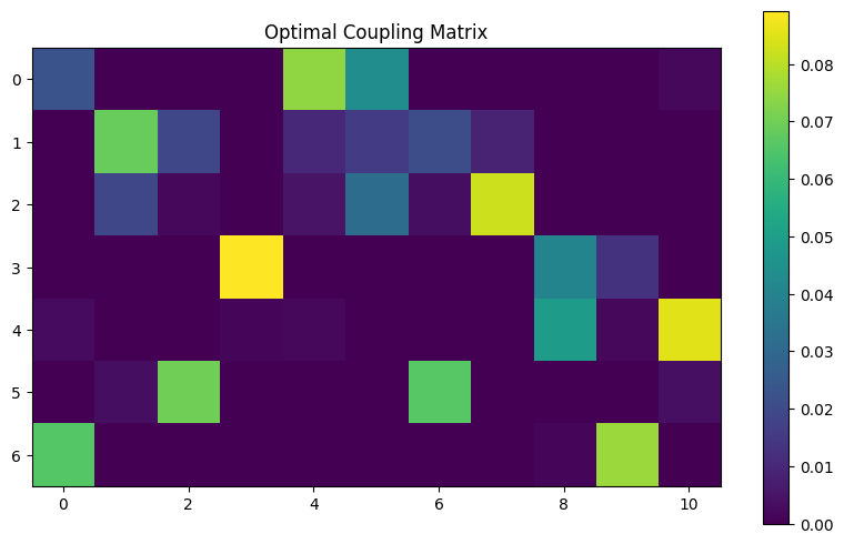
ot is a SinkhornOutput object that stores many more things, notably a lower, as well as an upper bound of the “true” squared 2-Wasserstein metric between x and y (the gap between these two bounds can be made arbitrarily small as epsilon decreases, when geom is instantiated).
print(
    f"2-Wasserstein: Lower bound = {ot.dual_cost:3f}, upper = {ot.primal_cost:3f}"
)
2-Wasserstein: Lower bound = 0.596925, upper = 1.038265
Automatic differentiation using jax#
We finish this quick tour by illustrating one of the main features of ott: it can be seamlessly integrated into differentiable, end-to-end architectures built using jax (see also Sinkhorn Divergence Hessians) for an example exploiting implicit differentiation).
We provide a simple use-case where we differentiate the (regularized) OT transport cost w.r.t. x,
by defining a wrapper that takes x and y as input, to output their regularized OT cost.
def reg_ot_cost(x: jnp.ndarray, y: jnp.ndarray) -> float:
    geom = pointcloud.PointCloud(x, y)
    ot = linear.solve(geom)
    return ot.reg_ot_cost
Obtaining the gradient function of reg_ot_cost is as easy as making a call to jax.grad() on reg_ot_cost, e.g. jax.grad(reg_ot_cost).
We use jax.value_and_grad() below to also store the value of the output itself. Note that by default, JAX only computes the gradient w.r.t the first of variable of reg_ot_cost , here x.
# value and gradient *function*
r_ot = jax.value_and_grad(reg_ot_cost)
# evaluate it at `(x, y)`.
cost, grad_x = r_ot(x, y)
assert grad_x.shape == x.shape
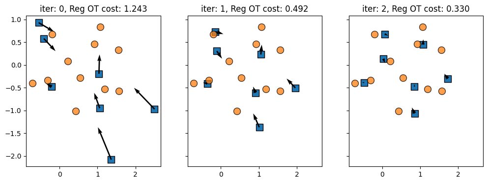
grad_x is a matrix that has the same size as x. Updating x with the opposite of that gradient decreases the loss. This process can done iteratively, following a gradient flow, to push x closer to y.
step = 2.0
x_t = x
quiv_args = {"scale": 1, "angles": "xy", "scale_units": "xy", "width": 0.01}
f, axes = plt.subplots(1, 3, sharey=True, sharex=True, figsize=(12, 4))

for iteration, ax in enumerate(axes):
    cost, grad_x = r_ot(x_t, y)
    ax.scatter(x_t[:, 0], x_t[:, 1], **x_args)
    ax.quiver(
        x_t[:, 0],
        x_t[:, 1],
        -step * grad_x[:, 0],
        -step * grad_x[:, 1],
        **quiv_args,
    )
    ax.scatter(y[:, 0], y[:, 1], **y_args)
    ax.set_title(f"iter: {iteration}, Reg OT cost: {cost:.3f}")
    x_t -= step * grad_x
Going further#
This tutorial gave you a glimpse of the most basic features of ott and how they integrate with jax.
ott implements many more functionalities, that are described in the following tutorials:
Seamless integration of other or even custom cost-functions in Point Clouds,
Better performance of
Sinkhornsolvers using various acceleration techniques in Focus on SinkhornExtensions of that approach to Gromov-Wasserstein, to compare distributions defined on heterogeneous spaces (for which a
cost_fn\(c(x,y)\) cannot be easily defined).Low-rank Sinkhorn for faster solvers that constraint coupling matrices (see plot above) to have a low-rank factorization, and exploit low-rank properties of {class}
Geometryobjects, both for the standard OT problem and its GW variant in Low-Rank GW.Wasserstein barycenters, as in GMM Barycenters or Sinkhorn Barycenters,
Differentiable sorting in Soft Sorting,
Neural solvers in Neural Dual Solver, to estimate maps in functional form.
Visual interface to plot progress bars in Tracking progress of ott.solvers.