Sinkhorn divergence gradient flows

Let \(\mathrm{OT_\varepsilon}(\alpha, \beta)\) the entropic regularized OT distance between two distributions \(\alpha\) and \(\beta\). One issue with \(\mathrm{OT_\varepsilon}\) is that \(\mathrm{OT_\varepsilon}(\alpha, \alpha)\) is not equal to 0.

The Sinkhorn divergence, defined in [Genevay et al., 2018] as \(\mathrm{S}_\varepsilon(\alpha, \beta) = \mathrm{OT_\varepsilon}(\alpha, \beta) - \frac{1}{2}\mathrm{OT_\varepsilon}(\alpha, \alpha) - \frac{1}{2}\mathrm{OT_\varepsilon}(\beta, \beta)\) removes this entropic bias.

In this tutorial we showcase the advantage of removing the entropic bias using gradient flows on 2-D distributions, as done in [Feydy et al., 2019] and following the Point Clouds tutorial.

Imports

import sys

if "google.colab" in sys.modules:
    !pip install -q git+https://github.com/ott-jax/ott@main

import jax
import jax.numpy as jnp

import matplotlib.pyplot as plt
from IPython import display

import ott
from ott.geometry import pointcloud
from ott.problems.linear import linear_problem
from ott.solvers.linear import sinkhorn
from ott.tools import plot, sinkhorn_divergence

/Users/michal/.mambaforge/envs/ott/lib/python3.10/site-packages/flax/struct.py:136: FutureWarning: jax.tree_util.register_keypaths is deprecated, and will be removed in a future release. Please use `register_pytree_with_keys()` instead.
  jax.tree_util.register_keypaths(data_clz, keypaths)
/Users/michal/.mambaforge/envs/ott/lib/python3.10/site-packages/flax/struct.py:136: FutureWarning: jax.tree_util.register_keypaths is deprecated, and will be removed in a future release. Please use `register_pytree_with_keys()` instead.
  jax.tree_util.register_keypaths(data_clz, keypaths)

Defining two distributions

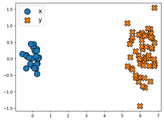
Let us start by defining simple source and target distributions.

key1, key2 = jax.random.split(jax.random.PRNGKey(0), 2)

x = 0.25 * jax.random.normal(key1, (25, 2))  # Source
y = 0.5 * jax.random.normal(key2, (50, 2)) + jnp.array((6, 0))  # Target

plt.scatter(x[:, 0], x[:, 1], edgecolors="k", marker="o", label="x", s=200)
plt.scatter(y[:, 0], y[:, 1], edgecolors="k", marker="X", label="y", s=200)
plt.legend(fontsize=15)
plt.show()

Gradient flow with \(\mathrm{OT}_\varepsilon\)

As in the Point Clouds tutorial, we now compute the gradient flow for the regularized OT cost using the Sinkhorn algorithm.

The code below performs gradient descent to move the points of \(x\) in a way that minimizes the regularized OT cost.

def gradient_flow(
    x: jnp.ndarray,
    y: jnp.ndarray,
    cost_fn: callable,
    num_iter: int = 500,
    lr: float = 0.2,
    dump_every: int = 50,
    epsilon: float = None,
):
    """Compute a gradient flow."""

    ots = []

    # Apply jax.value_and_grad operator and jit that function.
    cost_fn_vg = jax.jit(jax.value_and_grad(cost_fn, has_aux=True))

    # Perform gradient descent on `x`.
    for i in range(0, num_iter + 1):
        # Define the geometry, then compute the OT cost and its gradient.
        geom = pointcloud.PointCloud(x, y, epsilon=epsilon)
        (cost, ot), geom_g = cost_fn_vg(geom)
        assert ot.converged

        x = x - geom_g.x * lr  # Perform a gradient descent step.
        if i % dump_every == 0:
            ots.append(ot)  # Save the current state of the optimization.

    return ots

def display_animation(ots, plot_class=plot.Plot):
    """Display an animation of the gradient flow."""
    plott = plot_class(show_lines=False)
    anim = plott.animate(ots, frame_rate=4)
    html = display.HTML(anim.to_jshtml())
    display.display(html)
    plt.close()

def reg_ot_cost(geom):
    """Return the OT cost and OT output given a geometry"""
    ot = sinkhorn.Sinkhorn()(linear_problem.LinearProblem(geom))
    return ot.reg_ot_cost, ot

For the default value of \(\varepsilon\), the gradient flow behaves as expected:

# Compute and display the gradient flow for the regularized OT cost.
ots = gradient_flow(x, y, reg_ot_cost)
display_animation(ots)

Once Loop Reflect

But for a larger \(\varepsilon\), the distribution collapses:

# Compute and display the gradient flow for a larger value of epsilon.
ots = gradient_flow(x, y, reg_ot_cost, epsilon=1.0)
display_animation(ots)

Once Loop Reflect