Sinkhorn Divergence Hessians

In this tutorial, we showcase the ability of OTT to differentiate automatically its outputs. We highlight this by computing the Hessian of the sinkhorn_divergence() w.r.t. either weights a of the input measure, or locations x. Two approaches can be used to do so: rely on JAX native handling of computational graphs, or by using instead implicit differentiation of the solutions computed by OTT. In the example below we show that they are equivalent, but note this may not always be the case.

import sys

if "google.colab" in sys.modules:
    %pip install -q git+https://github.com/ott-jax/ott@main

import jax
import jax.numpy as jnp

import matplotlib.pyplot as plt

from ott.geometry import pointcloud
from ott.solvers.linear import implicit_differentiation as imp_diff
from ott.tools import sinkhorn_divergence

def sample(n: int, m: int, dim: int):
    """Sample points and random perturbation directions."""
    rngs = jax.random.split(jax.random.PRNGKey(0), 7)
    x = jax.random.uniform(rngs[0], (n, dim))
    y = jax.random.uniform(rngs[1], (m, dim))
    a = jax.random.uniform(rngs[2], (n,)) + 0.1
    b = jax.random.uniform(rngs[3], (m,)) + 0.1
    a = a / jnp.sum(a)
    b = b / jnp.sum(b)
    delta_a = jax.random.uniform(rngs[5], (n,)) - 0.5
    delta_a = delta_a - jnp.mean(delta_a)  # sums to 0.
    delta_x = jax.random.uniform(rngs[6], (n, dim)) - 0.5

    return a, x, b, y, delta_a, delta_x

Sample two random 3-dimensional point clouds and their perturbations.

a, x, b, y, delta_a, delta_x = sample(17, 15, 3)

As usual in JAX, we define a custom loss that outputs the quantity of interest, and is defined using relevant inputs as arguments, i.e. parameters against which we may want to differentiate. We add to a and x the implicit auxiliary flag which will be used to switch between unrolling and implicit differentiation of the Sinkhorn algorithm (see this excellent tutorial for a deep dive on their differences).

The loss outputs the Sinkhorn divergence between two point clouds.

def loss(a: jnp.ndarray, x: jnp.ndarray, implicit: bool = True) -> float:
    return sinkhorn_divergence.sinkhorn_divergence(
        pointcloud.PointCloud,
        x,
        y,  # this part defines geometry
        a=a,
        b=b,  # this sets weights
        sinkhorn_kwargs={
            "implicit_diff": imp_diff.ImplicitDiff() if implicit else None,
            "use_danskin": False,
        },
    ).divergence

Let’s parse the above call to sinkhorn_divergence() above:

• The first three lines define the point cloud geometry between x and y that will define the cost matrix. Here we could have added details on epsilon regularization (or scheduler), as well as alternative definitions of the cost function (here assumed by default to be squared Euclidean distance). We stick to the default setting.

• The next two lines set the respective weight vectors a and b. Those are simply two histograms of size n and m, both sum to \(1\), in the so-called balanced setting.

• Lastly, sinkhorn_kwargs pass arguments to three Sinkhorn solvers that will be called to compare x with y, x with x and y with y with their respective weights a and b. Rather than focusing on the several numerical options available to parameterize Sinkhorn’s behavior, we instruct JAX on how it should differentiate the outputs of the Sinkhorn algorithm. The use_danskin flag specifies whether the outputted potentials should be frozen when differentiating. Since we aim for second-order differentiation here, we must set this to False (if we wanted to compute gradients, True would have resulted in faster yet almost equivalent computations).

Computing Hessians

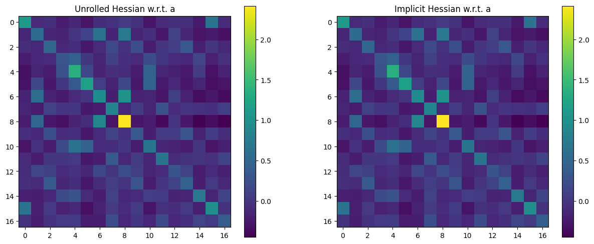
Let’s now plot Hessians of this output w.r.t. either a or x.

• The Hessian w.r.t. a will be a \(n \times n\) matrix, with the convention that a has size \(n\). Note that this Hessian matrix should be, in principle, positive definite. This is a property we check numerically.

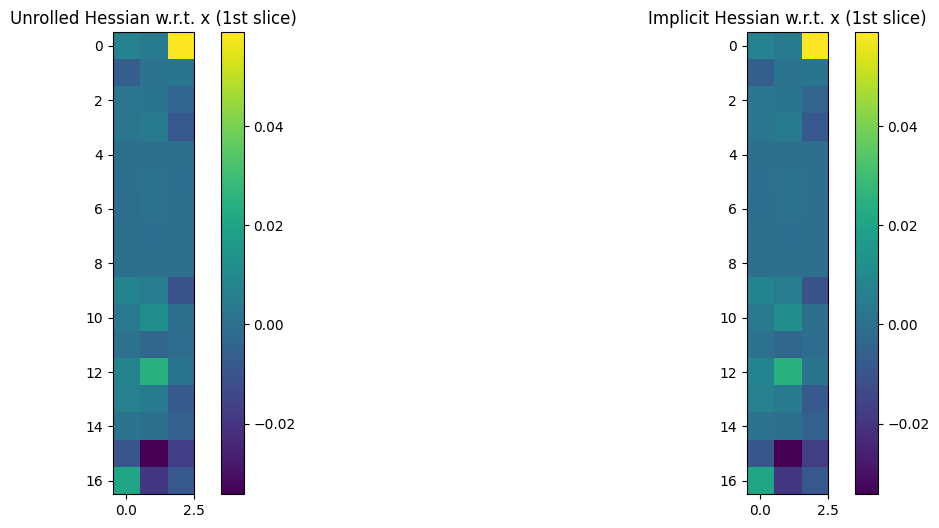
• Because x is itself a matrix of 3D coordinates, the Hessian w.r.t. x will be a 4D tensor of size \(n \times 3 \times n \times 3\).

To plot both Hessians, we loop on arg \(0\) (corresponding to a) or \(1\) (corresponding to x) of loss, and plot all (or part, for x) of those Hessian operators, to check they match. We only plot a thin \(n\times 3\) slice of the 4D tensor for x. We also check numerically that these Hessian operators are sound when compared to a finite difference approximation applied on an arbitrary direction.

# Loop over differentiating w.r.t. weights `a` or locations `x`.
for arg in [0, 1]:
    print(
        "Derivation w.r.t. " + ("weights `a`" if arg == 0 else "locations `x`")
    )
    fig, (ax1, ax2) = plt.subplots(1, 2, figsize=(15, 6))
    # Materialize Hessians using either implicit or unrolling.
    hessians = {}
    methods = ("Unrolled", "Implicit")
    for imp, method, axs in zip((False, True), methods, (ax1, ax2)):
        hess_loss = jax.jit(
            jax.hessian(lambda a, x: loss(a, x, imp), argnums=arg)
        )
        print("---- Time: " + method + " Hessian")
        %timeit _ = hess_loss(a, x).block_until_ready()
        hess = hess_loss(a, x)
        if arg == 0:
            # Because the OT problem is balanced, Hessians w.r.t. weights are
            # only defined up to the orthogonal space of 1s.
            # For that reason we remove that contribution to compare the properties
            # of these matrices.
            hess -= jnp.mean(hess, axis=1)[:, None]

            # We now look into their eigenvalues to check they are all nonnegative.
            eigenvalues = jnp.real(jnp.linalg.eig(hess)[0])
            e_min, e_max = jnp.min(eigenvalues), jnp.max(eigenvalues)
            print(
                "Min | Max eigenvalues of Hessian-",
                method,
                " ",
                e_min,
                " | ",
                e_max,
            )

        # Plot Hessian Matrix (or 2D slice if 4D tensor)
        im = axs.imshow(hess if arg == 0 else hess[0, 0, :, :])
        axs.set_title(
            method + " Hessian w.r.t. " + ("a" if arg == 0 else "x (1st slice)")
        )
        fig.colorbar(im, ax=axs)
        hessians[method] = hess

    # Comparison with Finite differences
    delta = delta_x if arg else delta_a

    # Compute <delta, H delta> where H is either unrolled/implicit Hessian
    diffs = {}
    for method, hess_mat in hessians.items():
        if arg == 0:
            h_d = hess_mat @ delta
        else:
            h_d = jnp.tensordot(hess_mat, delta)
        diffs[method] = jnp.sum(delta * h_d)

    # Approx <delta, H delta> using finite differences.
    a_p, a_m, x_p, x_m = a, a, x, x
    perturb_scale = 1e-3
    if arg == 0:
        a_p = a + perturb_scale * delta
        a_m = a - perturb_scale * delta
    else:
        x_p = x + perturb_scale * delta
        x_m = x - perturb_scale * delta

    app_p = loss(a_p, x_p)
    app_m = loss(a_m, x_m)
    fin_dif = (app_p + app_m - 2 * loss(a, x)) / (perturb_scale**2)

    # Print them to check they are relatively close.
    print("---- Hessian quadratic form at random perturbation")
    for m in methods:
        print(m + " Diff. :" + str(diffs[m]))
    print("Finite Diff. :", fin_dif, "\n")

Derivation w.r.t. weights `a`
---- Time: Unrolled Hessian
1.99 ms ± 92.7 µs per loop (mean ± std. dev. of 7 runs, 1 loop each)
Min | Max eigenvalues of Hessian- Unrolled   9.099584e-07  |  3.53894
---- Time: Implicit Hessian
2.38 ms ± 164 µs per loop (mean ± std. dev. of 7 runs, 1 loop each)
Min | Max eigenvalues of Hessian- Implicit   -2.0220386e-07  |  3.539016
---- Hessian quadratic form at random perturbation
Unrolled Diff. :0.9277187
Implicit Diff. :0.9277266
Finite Diff. : 0.9536743 

Derivation w.r.t. locations `x`
---- Time: Unrolled Hessian
8.48 ms ± 82.3 µs per loop (mean ± std. dev. of 7 runs, 1 loop each)
---- Time: Implicit Hessian
7.13 ms ± 205 µs per loop (mean ± std. dev. of 7 runs, 1 loop each)
---- Hessian quadratic form at random perturbation
Unrolled Diff. :-0.21479894
Implicit Diff. :-0.21479797
Finite Diff. : -0.23841858