Meta OT

This tutorial covers how to learn a Meta OT initializer for Sinkhorn [Amos et al., 2022] to help predict a reasonable initialization, and along the way we will also show how to use a Gaussian initializer [Thornton and Cuturi, 2022]. These initialization schemes can greatly speed-up the convergence of Sinkhorn algorithm, which otherwise usually starts from a zero initialization. Deploying optimal transport methods often involves having to solve many similar OT problems. While Sinkhorn can be run independently on the problems, to solve them from scratch, Meta OT methods argue that the runtime of the solver can be significantly improved by learning about the shared structure between the problem instances and using it to predict an approximate starting point that can be further refined.

We will cover:

• MetaInitializer: The main class for the Meta OT initializer

• GaussianInitializer: The main initialization class for the Gaussian initializer

Setup and helper functions

import sys

if "google.colab" in sys.modules:
    %pip install -q git+https://github.com/ott-jax/ott@main
    %pip install -q torch torchvision

from collections import namedtuple

import jax
import jax.numpy as jnp
import numpy as np
import torchvision

from flax import linen as nn

import matplotlib.pyplot as plt
from matplotlib import cm

from ott.geometry import pointcloud
from ott.initializers.linear import initializers
from ott.initializers.neural import meta_initializer
from ott.problems.linear import linear_problem
from ott.solvers.linear import sinkhorn

# Obtain the MNIST dataset and flatten the images into discrete measures.


def get_mnist_flat(train):
    dataset = torchvision.datasets.MNIST(
        "/tmp/mnist/",
        download=True,
        train=train,
    )
    data = jnp.array(dataset.data)
    data = data / 255.0
    data = data.reshape(-1, 784)
    data = data / data.sum(axis=1, keepdims=True)
    return data


mnist_train_data = get_mnist_flat(True)
mnist_eval_data = get_mnist_flat(False)

# Set up the geometry to use the grid of pixels
sinkhorn_epsilon = 1e-2
x_grid = []
for i in jnp.linspace(1, 0, num=28):
    for j in jnp.linspace(0, 1, num=28):
        x_grid.append([j, i])
x_grid = jnp.array(x_grid)
geom = pointcloud.PointCloud(x=x_grid, epsilon=sinkhorn_epsilon)

# Sample pairs of flattened MNIST digits
OT_Pair = namedtuple("OT_Pair", "a b")


def sample_OT_pairs(key, batch_size=128, train=True):
    data = mnist_train_data if train else mnist_eval_data
    k1, k2, key = jax.random.split(key, num=3)
    I = jax.random.randint(k1, shape=[batch_size], minval=0, maxval=len(data))
    J = jax.random.randint(k2, shape=[batch_size], minval=0, maxval=len(data))
    a = data[I]
    b = data[J]
    return OT_Pair(a, b)


# Generate an interpolation between the measures by sampling from the transport map.
def interpolate(
    key,
    f,
    g,
    a,
    b,
    num_interp_frames=8,
    title=None,
    axs=None,
    num_estimation_iterations=20,
    num_samples_marginal=1000,
):
    P = geom.transport_from_potentials(f, g)
    log_P_flat = jnp.log(P).ravel()

    @jax.jit
    def sample_interp_histogram_single(key, t):
        map_samples = jax.random.categorical(
            key, logits=log_P_flat, shape=[num_samples_marginal]
        )
        a_samples = geom.x[map_samples // len(a)]
        b_samples = geom.y[map_samples % len(a)]
        interp_samples = (1.0 - t) * a_samples + t * b_samples
        interp_hist, _, _ = jnp.histogram2d(
            interp_samples[:, 1],
            interp_samples[:, 0],
            bins=jnp.linspace(0.0, 1.0, num=28 + 1),
        )
        interp_hist = jnp.flipud(interp_hist)
        return interp_hist

    def sample_interp_histogram(key, t):
        alpha_t = 0.0
        for _ in range(num_estimation_iterations):
            k1, key = jax.random.split(key)
            alpha_t += sample_interp_histogram_single(k1, t)
        alpha_t = np.array(alpha_t)
        thresh = np.quantile(alpha_t, 0.95)
        alpha_t[alpha_t > thresh] = thresh
        return alpha_t / alpha_t.max()

    if axs is None:
        nrow, ncol = 1, num_interp_frames
        fig, axs = plt.subplots(
            nrow,
            ncol,
            figsize=(1 * ncol, 1 * nrow),
            gridspec_kw={"wspace": 0, "hspace": 0},
            dpi=80,
        )

    for i, t in enumerate(jnp.linspace(0, 1, num=num_interp_frames)):
        k1, key = jax.random.split(key)
        alpha_t = sample_interp_histogram(k1, t)
        axs[i].imshow(alpha_t.reshape(28, 28), cmap=cm.Greys)

    for ax in axs:
        ax.set_xticks([])
        ax.set_yticks([])

    if title is not None:
        fig.suptitle(title, y=1.2, fontsize=20)

Setting: optimal transport between pairs of MNIST digits

Computing the OT map between images provides a way of connecting their pixel intensities. For example, the OT distance between MNIST digits can be used for classification [Cuturi, 2013], which we will focus on in this tutorial.

Transporting between pairs of MNIST digits is a setting where the OT map needs to be repeatedly computed between every pair of digits. The standard use of optimal transport for solving these coupling problems is to treat every problem independently and solve each one from scratch. This is inefficient as similar problem instances, especially between similar digits, have similar solutions and transport maps.

Meta OT [Amos et al., 2022] is a way of learning this shared structure. This tutorial shows how to train a meta OT model to predict the optimal Sinkhorn potentials from the image pairs. We will reproduce their results using MetaInitializer, which provides an easy-to-use interface for training and using Meta OT models.

We consider each MNIST digit (a \(28 \times 28\) grayscale image) as a discrete distribution with fixed support as pixel coordinates and the weights are the normalized pixel intensity values corresponding to the pixel coordinate for each digit. Hence, \(x\) and \(y\) correspond to pixel coordinates, and each digit corresponds to a discrete distribution with support of size \(n_a=n_b=28\cdot28=784\).

The next block shows how our sampling function can be used to obtain batches of pairs of MNIST evaluation images.

key = jax.random.PRNGKey(0)
num_samples = 8
demo_batch = sample_OT_pairs(key, batch_size=num_samples, train=False)

nrow, ncol = 2, num_samples
fig, axs = plt.subplots(
    nrow,
    ncol,
    figsize=(1 * ncol, 1 * nrow),
    gridspec_kw={"wspace": 0, "hspace": 0},
    dpi=80,
)

for batch_idx in range(ncol):
    axs[0, batch_idx].imshow(
        demo_batch.a[batch_idx].reshape(28, 28), cmap=cm.Greys
    )
    axs[1, batch_idx].imshow(
        demo_batch.b[batch_idx].reshape(28, 28), cmap=cm.Greys
    )

for ax in axs.ravel():
    ax.set_xticklabels([])
    ax.set_yticklabels([])
    ax.set_xticks([])
    ax.set_yticks([])
axs[0, 0].set_ylabel(r"$\alpha$", rotation=0, size=24)
axs[0, 0].yaxis.set_label_coords(-0.2, 0.3)
axs[1, 0].set_ylabel(r"$\beta$", rotation=0, size=24)
axs[1, 0].yaxis.set_label_coords(-0.2, 0.3)

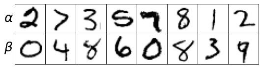
Coupling MNIST digits with Sinkhorn

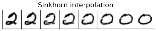
We interpret the pair of MNIST digits as discrete measures \(\alpha = \sum_{i=1}^{n_a} a_i \delta_{x_i}\) and \(\beta = \sum_{j=1}^{n_b} b_j \delta_{y_j}\). The default Sinkhorn implementation in Sinkhorn can easily compute their optimal coupling and associated dual potentials \(f\) and \(g\) from scratch. The optimal coupling between the measures can be used to generate an OT interpolation which shows how the measures are connected.

This next block solves the discrete LinearProblem associated with the first instance of the batch above with Sinkhorn and visualizes the OT interpolation. Given the optimal transport map \(P^\star\), the interpolation shows

\[\alpha_t = (t{\rm proj}_y+(1-t){\rm proj}_x) _{\#}P^\star\]

where \(t\in [0,1]\), \({\rm proj}_x(x,y):= x\), and \({\rm proj}_y(x,y):= y\).

a, b = demo_batch.a[0], demo_batch.b[0]
prob = linear_problem.LinearProblem(geom, a=a, b=b)

solver = sinkhorn.Sinkhorn()

base_sink_out = solver(prob)
interpolate(
    key, base_sink_out.f, base_sink_out.g, a, b, title="Sinkhorn interpolation"
)

Meta Optimal Transport

For discrete OT, Meta OT [Amos et al., 2022] predicts the optimal dual variables \(f^\star\) from the input measures \(\alpha,\beta\) and geometry, which can then map to \(g^\star\) and the transport map \(P^\star\):

Meta OT’s objective based amortization.

We will consider a model \(\hat f_\theta(a, b)\) that predicts the duals given the probabilities of the measures, i.e. \(a\) and \(b\), leaving the geometry (and cost) fixed. The MNIST measures fit into this setting because the pixel locations remain fixed.

Learning the model. The goal is for the model to match the optimal duals, i.e., \(\hat f_\theta \approx f^\star\). This can be done by training the predictions of \(f_\theta\) to optimize the dual objective, which \(f^\star\) also optimizes for. The overall learning setup can thus be written as:

\[\min_\theta\; {\mathbb E}_{(\alpha,\beta)\sim{\mathcal{D}}}\; J(\hat f_\theta(a, b); \alpha, \beta),\]

where \(a,b\) are the probabilities of the measures \(\alpha,\beta\), \(\mathcal{D}\) is some distribution of optimal transport problems, and

\[-J(f; \alpha, \beta, c) := \langle f, a\rangle + \langle g, b \rangle - \varepsilon\left\langle \exp\{f/\varepsilon\}, K\exp\{g/\varepsilon\}\right\rangle\]

is the entropic dual objective, and \(K_{i,j} := -C_{i,j}/\varepsilon\) is the Gibbs kernel. Notably, this loss doesn’t require access to the ground-truth \(f^\star\) and instead locally updates the predictions. In other words, the Meta OT model simultaneously solves all of the OT problems in the meta distribution \(\mathcal{D}\) during training

The following instantiates MetaInitializer, which provides an implementation for training and deploying Meta OT models. The default meta potential model for \(f_\theta\) is a standard multi-layer MLP defined by the MetaMLP below and it is optimized with adam() by default.

Custom model and optimizers. The model and training procedure use flax and optax. The Meta OT initializer can take a custom-written Flax module in init_model or optimizer in opt that may be better-suited to your setting than an MLP.

Creating the initializer

We can create the initializer by providing it with the shared geometry of the problem instances. First, we create an MLP, which takes in the concatenated \(\alpha\) and \(\beta\) probability measures and outputs the potential.

class MetaMLP(nn.Module):
    potential_size: int
    num_hidden_units: int = 512
    num_hidden_layers: int = 3

    @nn.compact
    def __call__(self, z: jnp.ndarray) -> jnp.ndarray:
        for _ in range(self.num_hidden_layers):
            z = nn.relu(nn.Dense(self.num_hidden_units)(z))

        return nn.Dense(self.potential_size)(z)

meta_mlp = MetaMLP(potential_size=geom.shape[0])
meta_initializer = meta_initializer.MetaInitializer(
    geom=geom, meta_model=meta_mlp
)

Training the Meta OT initializer

Meta OT models have a preliminary training phase where they are given samples of OT problems from the meta distribution. The Meta OTT initializer internally stores the training state of the model, and update() will update the initialization on a batch of problems to improve the next prediction. While we show here a separate training phase, the update can also be done in-tandem with deployment where the initialization is then used with a Sinkhorn refinement process to obtain optimal solutions. This is appealing for deployment settings because even if the Meta OT model is suboptimal, refining the prediction with Sinkhorn is guaranteed to provide an optimal solution to the transport problem.

num_train_iterations = 50_000

for train_iter in range(num_train_iterations):
    key, step_key = jax.random.split(key)
    batch = sample_OT_pairs(step_key, train=True)
    loss, init_f, meta_initializer.state = meta_initializer.update(
        meta_initializer.state, a=batch.a, b=batch.b
    )
    print(f"Train iteration: {train_iter+1} - Loss: {loss:.2e}", end="\r")

Train iteration: 50000 - Loss: -3.54e-02

Training complete!

Now that we have trained the model, we can next deploy it anytime we want to make a rough prediction for new instances of the problems. While in practice, the model can be continued to be updated in deployment by calling update(), here we will keep the model fixed so we can evaluate it on test instances.

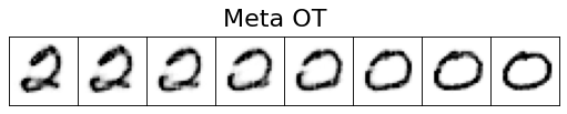
Visualizing the initializations

We can visualize the interpolation provided by the Meta OT model’s prediction of the solution to the transport problems from above, which are sampled from testing pairs of MNIST digits that the model was not trained on. The initializer uses the Meta OT model in init_dual_a(). This shows that the initialization is extremely close to the ground-truth coupling.

a, b = demo_batch.a[0], demo_batch.b[0]
ot_problem = linear_problem.LinearProblem(geom, a, b)

# Predict the optimal f duals.
f = meta_initializer.init_dual_a(ot_problem, lse_mode=True)

# Obtain the optimal g duals from the prediction.
g = geom.update_potential(f, jnp.zeros_like(b), jnp.log(b), 0, axis=0)

interpolate(key, f, g, a, b, title="Meta OT")

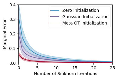
Evaluating the initializers

We lastly compare how much the initializers help Sinkhorn converge on these problems, measured by the marginal error:

\[{\rm err}(f,g; \alpha, \beta, c) := \|P1_m-a\|_1 + \|P^\top1_n-b\|_1\]

def get_errors(sink_out):
    return sink_out.errors[sink_out.errors > -1]


error_log = {"gaus": [], "base": [], "meta_ot": []}

num_evals = 10
eval_batch = sample_OT_pairs(
    jax.random.PRNGKey(0), batch_size=num_evals, train=False
)
for i in range(num_evals):
    a = eval_batch.a[i]
    b = eval_batch.b[i]

    sink_kwargs = {
        "threshold": -1,
        "inner_iterations": 1,
        "max_iterations": 26,
    }

    ot_problem = linear_problem.LinearProblem(geom, a=a, b=b)
    solver = sinkhorn.Sinkhorn(**sink_kwargs)

    base_sink_out = solver(ot_problem, init=(None, None))

    init_dual_a = meta_initializer.init_dual_a(ot_problem, lse_mode=True)
    meta_sink_out = solver(ot_problem, init=(init_dual_a, None))

    init_dual_a = initializers.GaussianInitializer().init_dual_a(
        ot_problem, lse_mode=True
    )
    gaus_sink_out = solver(ot_problem, init=(init_dual_a, None))

    error_log["base"].append(base_sink_out.errors)
    error_log["meta_ot"].append(meta_sink_out.errors)
    error_log["gaus"].append(gaus_sink_out.errors)

error_log = {key: jnp.array(errors) for (key, errors) in error_log.items()}

fig, ax = plt.subplots(figsize=(4, 2.5), dpi=100)
tag_map = {
    "meta_ot": "Meta OT Initialization",
    "gaus": "Gaussian Initialization",
    "base": "Zero Initialization",
}

bmh_colors = plt.style.library["bmh"]["axes.prop_cycle"].by_key()["color"]
colors = [bmh_colors[0], bmh_colors[2], bmh_colors[1]]
for tag, color in zip(["base", "gaus", "meta_ot"], colors):
    mean_errors = jnp.mean(error_log[tag], axis=0)
    ax.plot(mean_errors, label=tag_map[tag], color=color)

    iters = np.arange(len(mean_errors))
    stds = jnp.std(error_log[tag], axis=0)
    ax.fill_between(
        iters, mean_errors - stds, mean_errors + stds, color=color, alpha=0.3
    )

ax.set_xlabel("Number of Sinkhorn Iterations")
ax.set_ylabel("Marginal Error")
ax.legend()
ax.set_xlim(0, 25)
ax.set_ylim(0, 0.4);