Sinkhorn Barycenters#

import sys

if "google.colab" in sys.modules:
    %pip install -q git+https://github.com/ott-jax/ott@main
    %pip install -q nilearn

import nilearn
from nilearn import datasets, image, plotting
from nilearn.image import get_data

import jax
import jax.numpy as jnp
import numpy as np

import matplotlib.pyplot as plt

from ott.geometry import costs, epsilon_scheduler, grid
from ott.problems.linear import barycenter_problem as bp
from ott.solvers.linear import discrete_barycenter as db

Import neuroimaging data using `nilearn`.#

We recover a few MRI data points…

n_subjects = 4
dataset_files = datasets.fetch_oasis_vbm(
    n_subjects=n_subjects,
)
gm_imgs = np.array(dataset_files.gray_matter_maps)

/home/michal/mambaforge/envs/ott/lib/python3.10/site-packages/nilearn/datasets/struct.py:850: UserWarning: `legacy_format` will default to `False` in release 0.11. Dataset fetchers will then return pandas dataframes by default instead of recarrays.
  warnings.warn(_LEGACY_FORMAT_MSG)

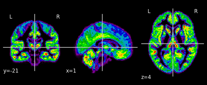
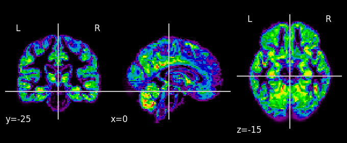
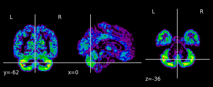
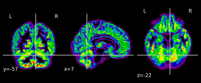
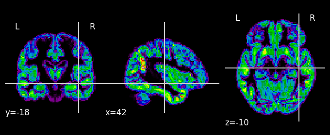
… and plot their gray matter densities.

for i in range(n_subjects):
    plotting.plot_epi(gm_imgs[i])
    plt.show()

../_images/54fad0783142c1438b62b95f2c46644cdead594579fc3881a700e939a0b376da.png

../_images/a392d282c64b7afec37998a6272183940ce85ac8c02beebabf04db20c98527b3.png

../_images/a9d1df1860c22119a32876eae2afde589aedebe1a7eac9b4475c7dab7dafbdef.png

../_images/1a35321f872eadf3412fb6f1bb95ba1ac68a7104c33af6f4b9941177dbeb64f5.png

Represent data as histograms#

We normalize those gray matter densities so that they sum to 1, and check their size.

a = jnp.array(get_data(gm_imgs)).transpose((3, 0, 1, 2))
grid_size = a.shape[1:4]
a = a.reshape((n_subjects, -1)) + 1e-2
a = a / np.sum(a, axis=1)[:, np.newaxis]
print("Grid size: ", grid_size)

Grid size:  (91, 109, 91)

Instantiate a grid geometry to compute \(W_p^p\)#

We instantiate the Grid geometry corresponding to these data points, living in a space of dimension \(91 \times 109 \times 91\), for a total total dimension \(d=902\ 629\). Rather than stretch these voxel histograms and put them in the \([0,1]^3\) hypercube, we use a simpler rescaled grid, \([0, 0.9] \times [0, 1.08] \times [0, 0.9]\), with increments of \(1/100\).

We endow points on that 3-dimensional grid with a custom cost function defined below: we use a \(p\)-norm, with \(p\) slighter larger than 1 following previous work of [Gramfort et al., 2015] on brain signals.

We use an \(\varepsilon\) scheduler that will decrease the regularization strength from \(0.1\) down to \(10^{-4}\) with a decay factor of \(0.95\).

@jax.tree_util.register_pytree_node_class
class Custom(costs.CostFn):
    """Custom function."""

    def pairwise(self, x, y):
        return jnp.sum(jnp.abs(x - y) ** 1.1)


# Instantiate Grid Geometry of suitable size, epsilon parameter and cost.
g_grid = grid.Grid(
    x=[jnp.arange(0, n) / 100 for n in grid_size],
    cost_fns=[Custom()],
    epsilon=epsilon_scheduler.Epsilon(target=1e-4, init=1e-1, decay=0.95),
)

Compute the regularized \(W_p^p\) iso-barycenter#

We jit and run the FixedBarycenter on the FixedBarycenterProblem.

%%time
solver = jax.jit(db.FixedBarycenter())
problem = bp.FixedBarycenterProblem(g_grid, a)
barycenter = solver(problem)

CPU times: user 7min 10s, sys: 4.43 s, total: 7min 15s
Wall time: 7min 1s

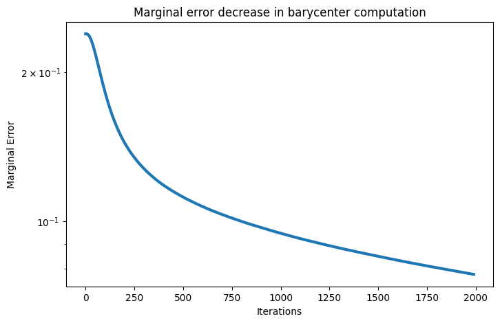
Plot decrease of marginal error#

The computation of the barycenter of \(N\) histograms involves the resolution of \(N\) OT problems pointing towards the same, but unknown, marginal [Benamou et al., 2015]. The convergence of that algorithm can be monitored by evaluating the distance between the marginals of these different transport matrices w.r.t. that same common marginal. Upon convergence that should be close to \(0\).

plt.figure(figsize=(8, 5))
errors = barycenter.errors[:-1]
plt.plot(np.arange(errors.size) * 10, errors, lw=3)
plt.title("Marginal error decrease in barycenter computation")
plt.yscale("log")
plt.xlabel("Iterations")
plt.ylabel("Marginal Error")
plt.show()

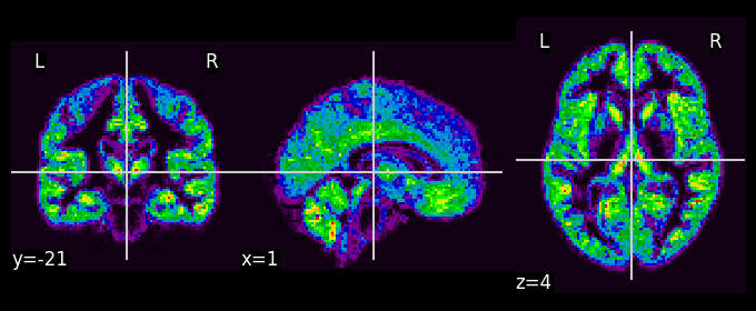
../_images/51d2a2cb87dc8385fa841632520d8f3748aa9471b9f366f171995cc83b569f25.png

Plot the barycenter itself#

def data_to_nii(x):
    return nilearn.image.new_img_like(
        gm_imgs[0], data=np.array(x.reshape(grid_size))
    )


plotting.plot_epi(data_to_nii(barycenter.histogram))
plt.show()

../_images/5d756193768f4a5eddf08989e03c7c0cd6dd363250a5611c0eb32ca4302ce0a2.png

SqEuclidean barycenter, for reference#

plotting.plot_epi(data_to_nii(np.mean(a, axis=0)))

<nilearn.plotting.displays._slicers.OrthoSlicer at 0x7f15970df280>

../_images/645671ba32c49a443b2c447636c4e9c2ec1c08e2e8f6dfb6cf57c1eda01ca093.png

Sinkhorn Barycenters

Contents