Expectile-Regularized OT

Expectile Regularization for Fast and Accurate Training of Neural Optimal Transport

The ExpectileNeuralDual solves the dual OT problem where the objective is a sum of Kantorovich potential functions with additional expectile regularization [Buzun et al., 2024]. The initialization arguments include:

• potential models that inherit from flax.linen.Module,

• a cost function of type CostFn,

• is_bidirectional boolean parameter that indicates whether we train the OT mapping in both directions,

• and two regularization parameters, expectile and expectile_loss_coef.

The training procedure returns the ENOTPotentials object that can be used to transport between input distributions or compute the corresponding OT distance between them.

import dataclasses
from collections.abc import Iterator, Mapping
from types import MappingProxyType
from typing import Any, Literal, Optional

import jax
import jax.numpy as jnp
import sklearn
import sklearn.datasets

import optax

import matplotlib.pyplot as plt
from IPython.display import clear_output, display

from ott import datasets
from ott.geometry import costs, pointcloud
from ott.neural.methods import expectile_neural_dual
from ott.neural.networks import potentials
from ott.tools import sinkhorn_divergence

Evaluation on synthetic 2D datasets

In this section we show how ENOT finds optimal map between two measures constructed from [Makkuva et al., 2020]. Here, we utilize create_gaussian_mixture_samplers() in order to get samples from source measure square_five and target measure square_four. In our experiments, we use a custom implementation of MLP for the potential models. Under the hood, the optimization is done with respect to the type of the cost function (e.g., SqEuclidean or PNormP).

num_samples_visualize = 512
(
    train_dataloaders,
    valid_dataloaders,
    input_dim,
) = datasets.create_gaussian_mixture_samplers(
    name_source="square_five",
    name_target="square_four",
    valid_batch_size=num_samples_visualize,
    train_batch_size=2048,
)

eval_data_source = next(valid_dataloaders.source_iter)
eval_data_target = next(valid_dataloaders.target_iter)

def plot_eval_samples(
    eval_data_source, eval_data_target, transported_samples=None
):
    fig, axs = plt.subplots(
        1, 2, figsize=(8, 4), gridspec_kw={"wspace": 0, "hspace": 0}
    )
    axs[0].scatter(
        eval_data_source[:, 0],
        eval_data_source[:, 1],
        color="#A7BED3",
        s=10,
        alpha=0.5,
        label="source",
    )
    axs[0].set_title("Source measure samples")
    axs[1].scatter(
        eval_data_target[:, 0],
        eval_data_target[:, 1],
        color="#1A254B",
        s=10,
        alpha=0.5,
        label="target",
    )
    axs[1].set_title("Target measure samples")

    if transported_samples is not None:
        axs[1].scatter(
            transported_samples[:, 0],
            transported_samples[:, 1],
            color="#F2545B",
            s=10,
            alpha=0.5,
            label="pushforward of source",
        )

    fig.legend(
        **{
            "ncol": (3 if transported_samples is not None else 2),
            "loc": "upper center",
            "bbox_to_anchor": (0.5, 0.1),
            "edgecolor": "k",
        }
    )

    for ax in axs:
        ax.set_xticks([])
        ax.set_yticks([])

    return fig, ax


fig, ax = plot_eval_samples(eval_data_source, eval_data_target)
display(fig)
plt.close(fig)

num_train_iters = 90_001


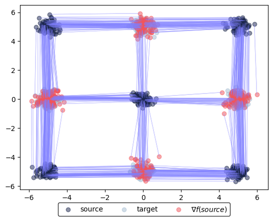
def training_callback(step, learned_potentials):
    if step % 2500 == 0:
        clear_output()
        print(f"Training iteration: {step}/{num_train_iters}")

        neural_dual_dist = learned_potentials.distance(
            eval_data_source, eval_data_target
        )
        print(
            f"Neural dual distance between source and target data: {neural_dual_dist:.2f}"
        )

        fig, ax = learned_potentials.plot_ot_map(
            eval_data_source,
            eval_data_target,
            forward=True,
        )
        display(fig)
        plt.close(fig)

        fig, ax = learned_potentials.plot_ot_map(
            eval_data_source,
            eval_data_target,
            forward=False,
        )
        display(fig)
        plt.close(fig)

Training

The main hyperparameters in ExpectileNeuralDual to look at are expectile and expectile_loss_coef, denoted in [Buzun et al., 2024] as \(\tau\) and \(\lambda\), respectively.

neural_f = potentials.LinenMLP(
    dim_hidden=[128, 128, 128, 128, 1], act_fn=jax.nn.elu
)
neural_g = potentials.LinenMLP(
    dim_hidden=[128, 128, 128, 128, 1], act_fn=jax.nn.elu
)

lr_schedule_f = optax.cosine_decay_schedule(
    init_value=5e-4, decay_steps=num_train_iters, alpha=1e-2
)

lr_schedule_g = optax.cosine_decay_schedule(
    init_value=5e-4, decay_steps=num_train_iters, alpha=1e-2
)
optimizer_f = optax.adam(learning_rate=lr_schedule_f, b1=0.9, b2=0.999)
optimizer_g = optax.adam(learning_rate=lr_schedule_g, b1=0.9, b2=0.999)

neural_dual_solver = expectile_neural_dual.ExpectileNeuralDual(
    input_dim,
    neural_f,
    neural_g,
    optimizer_f,
    optimizer_g,
    cost_fn=costs.SqEuclidean(),
    num_train_iters=num_train_iters,
    expectile=0.98,
    expectile_loss_coef=0.25,
    rng=jax.random.key(5),
)
learned_potentials = neural_dual_solver(
    *train_dataloaders,
    *valid_dataloaders,
    callback=training_callback,
)

Training iteration: 90000/90001
Neural dual distance between source and target data: 21.14

100%|███████████████████████████████████████████████████████████████████████████████████████████████████████████████████████████████| 90001/90001 [24:43<00:00, 60.68it/s]

Evaluation

@jax.jit
def sinkhorn_loss(
    x: jnp.ndarray, y: jnp.ndarray, epsilon: float = 0.001
) -> float:
    """Computes transport between (x, a) and (y, b) via Sinkhorn algorithm."""
    a = jnp.ones(len(x)) / len(x)
    b = jnp.ones(len(y)) / len(y)

    sdiv, _ = sinkhorn_divergence.sinkhorn_divergence(
        pointcloud.PointCloud, x, y, epsilon=epsilon, a=a, b=b
    )
    return sdiv

pred_target = learned_potentials.transport(eval_data_source)
print(
    f"Sinkhorn distance between target predictions and data samples: {sinkhorn_loss(pred_target, eval_data_target):.2f}"
)

pred_source = learned_potentials.transport(eval_data_target, forward=False)
print(
    f"Sinkhorn distance between source predictions and data samples: {sinkhorn_loss(pred_source, eval_data_source):.2f}"
)

neural_dual_dist = learned_potentials.distance(
    eval_data_source, eval_data_target
)
print(
    f"Neural dual distance between source and target data: {neural_dual_dist:.2f}"
)

sinkhorn_dist = sinkhorn_loss(eval_data_source, eval_data_target)
print(f"Sinkhorn distance between source and target data: {sinkhorn_dist:.2f}")

Sinkhorn distance between target predictions and data samples: 0.06
Sinkhorn distance between source predictions and data samples: 0.19
Neural dual distance between source and target data: 21.14
Sinkhorn distance between source and target data: 21.15

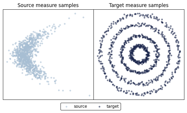
MAFMoons & Rings synthetic datasets

Below, we show how ENOT handles more challenging tasks. For this case, we implement the MAFMoonSampler and RingSampler data samplers.

@dataclasses.dataclass
class MAFMoonSampler:
    size: int

    def __iter__(self):
        rng = jax.random.key(0)
        while True:
            rng, sample_key = jax.random.split(rng, 2)
            yield self._sample(sample_key, self.size)

    def _sample(self, key, batch_size):
        x = jax.random.normal(key, shape=[batch_size, 2])
        x = x.at[:, 0].add(x[:, 1] ** 2)
        x = x.at[:, 0].mul(0.5)
        x = x.at[:, 0].add(-5)
        return x


@dataclasses.dataclass
class RingSampler:
    size: int

    def __iter__(self):
        rng = jax.random.key(0)
        while True:
            rng, sample_key = jax.random.split(rng, 2)
            yield self._sample(sample_key, self.size)

    def _sample(self, key, batch_size):
        n_samples4 = n_samples3 = n_samples2 = batch_size // 4
        n_samples1 = batch_size - n_samples4 - n_samples3 - n_samples2

        linspace4 = jnp.linspace(0, 2 * jnp.pi, n_samples4, endpoint=False)
        linspace3 = jnp.linspace(0, 2 * jnp.pi, n_samples3, endpoint=False)
        linspace2 = jnp.linspace(0, 2 * jnp.pi, n_samples2, endpoint=False)
        linspace1 = jnp.linspace(0, 2 * jnp.pi, n_samples1, endpoint=False)

        circ4_x = jnp.cos(linspace4) * 1.2
        circ4_y = jnp.sin(linspace4) * 1.2
        circ3_x = jnp.cos(linspace4) * 0.9
        circ3_y = jnp.sin(linspace3) * 0.9
        circ2_x = jnp.cos(linspace2) * 0.55
        circ2_y = jnp.sin(linspace2) * 0.55
        circ1_x = jnp.cos(linspace1) * 0.25
        circ1_y = jnp.sin(linspace1) * 0.25

        X = (
            jnp.vstack(
                [
                    jnp.hstack([circ4_x, circ3_x, circ2_x, circ1_x]),
                    jnp.hstack([circ4_y, circ3_y, circ2_y, circ1_y]),
                ]
            ).T
            * 3.0
        )
        X = sklearn.utils.shuffle(X)

        # Add noise
        X = X + jax.random.normal(key, shape=X.shape) * 0.08

        return X.astype("float32")

train_loader = datasets.Dataset(
    source_iter=iter(MAFMoonSampler(size=1024)),
    target_iter=iter(RingSampler(size=1024)),
)
valid_loader = train_loader

moon_samples = next(train_loader.source_iter)
ring_samples = next(train_loader.target_iter)

fig, ax = plot_eval_samples(moon_samples, ring_samples)
display(fig)
plt.close(fig)

eval_data_source = next(valid_loader.source_iter)
eval_data_target = next(valid_loader.target_iter)

neural_f = potentials.LinenMLP(
    dim_hidden=[128, 128, 128, 128, 1], act_fn=jax.nn.elu
)
neural_g = potentials.LinenMLP(
    dim_hidden=[128, 128, 128, 128, 1], act_fn=jax.nn.elu
)

num_train_iters = 90_001
lr_schedule_f = optax.cosine_decay_schedule(
    init_value=5e-4, decay_steps=num_train_iters, alpha=1e-3
)

lr_schedule_g = optax.cosine_decay_schedule(
    init_value=5e-4, decay_steps=num_train_iters, alpha=1e-3
)
optimizer_f = optax.adam(learning_rate=lr_schedule_f, b1=0.9, b2=0.999)
optimizer_g = optax.adam(learning_rate=lr_schedule_g, b1=0.9, b2=0.999)

neural_dual_solver = expectile_neural_dual.ExpectileNeuralDual(
    2,
    neural_f,
    neural_g,
    optimizer_f,
    optimizer_g,
    cost_fn=costs.SqEuclidean(),
    num_train_iters=num_train_iters,
    expectile=0.99,
    expectile_loss_coef=0.3,
    rng=jax.random.key(4),
)
learned_potentials = neural_dual_solver(*train_loader, *valid_loader)

100%|██████████████████████████████████████████████████████████████████████████████████████████████████████████████████████████████| 90001/90001 [11:12<00:00, 133.84it/s]

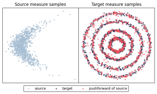
Evaluate the learned_potentials.

fig, ax = plot_eval_samples(
    moon_samples, ring_samples, learned_potentials.transport(moon_samples)
)
display(fig)
plt.close(fig)

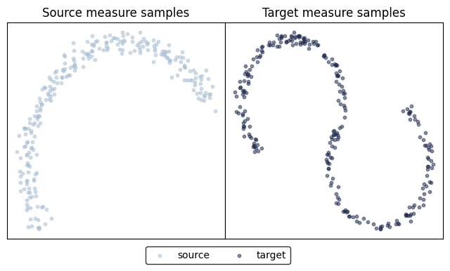
Different costs on 2D data

Next, we show how ENOT performs when varying the underlying cost function \(c(x, y)\) on synthetic 2D datasets HalfMoon and S_curve.

@dataclasses.dataclass
class SklearnDistribution:
    name: Literal["moon", "s_curve"]
    theta_rotation: float = 0.0
    mean: Optional[jnp.ndarray] = None
    noise: float = 0.01
    scale: float = 1.0
    batch_size: int = 1024
    rng: Optional[jax.Array] = None

    def __iter__(self) -> Iterator[jnp.ndarray]:
        return self._create_sample_generators()

    def _create_sample_generators(self) -> Iterator[jnp.ndarray]:
        rng = jax.random.key(0) if self.rng is None else self.rng
        rotation = jnp.array(
            [
                [jnp.cos(self.theta_rotation), -jnp.sin(self.theta_rotation)],
                [jnp.sin(self.theta_rotation), jnp.cos(self.theta_rotation)],
            ]
        )
        while True:
            rng, _ = jax.random.split(rng)
            seed = jax.random.randint(rng, [], minval=0, maxval=1e5).item()
            if self.name == "moon":
                samples, _ = sklearn.datasets.make_moons(
                    n_samples=(self.batch_size, 0),
                    random_state=seed,
                    noise=self.noise,
                )
            elif self.name == "s_curve":
                x, _ = sklearn.datasets.make_s_curve(
                    n_samples=self.batch_size,
                    random_state=seed,
                    noise=self.noise,
                )
                samples = x[:, [2, 0]]
            else:
                raise NotImplementedError(
                    f"SklearnDistribution `{self.name}` not implemented."
                )

            samples = jnp.asarray(samples, dtype=jnp.float32)
            samples = jnp.squeeze(jnp.matmul(rotation[None, :], samples.T).T)
            mean = jnp.zeros(2) if self.mean is None else self.mean
            samples = mean + self.scale * samples
            yield samples


def create_samplers(
    source_kwargs: Mapping[str, Any] = MappingProxyType({}),
    target_kwargs: Mapping[str, Any] = MappingProxyType({}),
    train_batch_size: int = 256,
    valid_batch_size: int = 256,
    rng: Optional[jax.Array] = None,
):
    rng = jax.random.key(0) if rng is None else rng
    rng1, rng2, rng3, rng4 = jax.random.split(rng, 4)
    train_dataset = datasets.Dataset(
        source_iter=iter(
            SklearnDistribution(
                rng=rng1, batch_size=train_batch_size, **source_kwargs
            )
        ),
        target_iter=iter(
            SklearnDistribution(
                rng=rng2, batch_size=train_batch_size, **target_kwargs
            )
        ),
    )
    valid_dataset = datasets.Dataset(
        source_iter=iter(
            SklearnDistribution(
                rng=rng3, batch_size=valid_batch_size, **source_kwargs
            )
        ),
        target_iter=iter(
            SklearnDistribution(
                rng=rng4, batch_size=valid_batch_size, **target_kwargs
            )
        ),
    )
    dim_data = 2
    return train_dataset, valid_dataset, dim_data

train_dataset, valid_dataset, dim_data = create_samplers(
    source_kwargs={
        "name": "moon",
        "theta_rotation": jnp.pi / 6,
        "mean": jnp.array([0.0, -0.5]),
        "noise": 0.05,
    },
    target_kwargs={
        "name": "s_curve",
        "scale": 0.6,
        "mean": jnp.array([0.5, -2.0]),
        "theta_rotation": -jnp.pi / 6,
        "noise": 0.05,
    },
)

train_source = next(train_dataset.source_iter)
train_target = next(train_dataset.target_iter)
fig, ax = plot_eval_samples(train_source, train_target)
display(fig)
plt.close(fig)

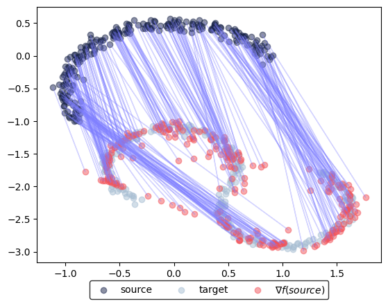
Squared-Euclidean cost

We change the cost to the SqEuclidean and visualize results:

neural_f = potentials.LinenMLP(dim_hidden=[64, 64, 64, 1], act_fn=jax.nn.gelu)
neural_g = potentials.LinenMLP(dim_hidden=[64, 64, 64, 1], act_fn=jax.nn.gelu)

num_train_iters = 50_001

lr_schedule_f = optax.cosine_decay_schedule(
    init_value=3e-4, decay_steps=num_train_iters, alpha=1e-4
)

lr_schedule_g = optax.cosine_decay_schedule(
    init_value=3e-4, decay_steps=num_train_iters, alpha=1e-4
)
optimizer_f = optax.adam(learning_rate=lr_schedule_f, b1=0.9, b2=0.999)
optimizer_g = optax.adam(learning_rate=lr_schedule_g, b1=0.9, b2=0.999)

neural_dual_solver = expectile_neural_dual.ExpectileNeuralDual(
    2,
    neural_f,
    neural_g,
    optimizer_f,
    optimizer_g,
    num_train_iters=num_train_iters,
    expectile=0.99,
    expectile_loss_coef=1,
    cost_fn=costs.SqEuclidean(),
    rng=jax.random.key(42),
)

sample_data_source = next(train_dataset.source_iter)
sample_data_target = next(train_dataset.target_iter)

learned_potentials = neural_dual_solver(
    *train_dataset, *valid_dataset, callback=training_callback
)

Training iteration: 50000/50001
Neural dual distance between source and target data: 5.11

100%|██████████████████████████████████████████████████████████████████████████████████████████████████████████████████████████████| 50001/50001 [02:16<00:00, 366.08it/s]

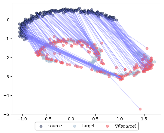
PNormP cost

Finally, we change the cost to the PNormP with \(p=1.5\):

neural_dual_solver = expectile_neural_dual.ExpectileNeuralDual(
    2,
    neural_f,
    neural_g,
    optimizer_f,
    optimizer_g,
    num_train_iters=num_train_iters,
    expectile=0.99,
    expectile_loss_coef=1,
    cost_fn=costs.PNormP(1.5),
    rng=jax.random.key(42),
)

sample_data_source = next(train_dataset.source_iter)
sample_data_target = next(train_dataset.target_iter)

learned_potentials = neural_dual_solver(
    *train_dataset, *valid_dataset, callback=training_callback
)

Training iteration: 50000/50001
Neural dual distance between source and target data: 2.63

100%|██████████████████████████████████████████████████████████████████████████████████████████████████████████████████████████████| 50001/50001 [02:24<00:00, 346.43it/s]