Multimarginal OT

We consider in this tutorial the resolution of the multimarginal OT problem, as first formulated in [Gangbo and Święch, 1998] and solved numerically in [Benamou et al., 2015] using entropic regularization. This algorithm serves as the main engine of the M3G loss presented in [Piran et al., 2024].

from typing import Optional

import jax
import jax.numpy as jnp

import matplotlib.pyplot as plt
from IPython import display
from matplotlib import colors

from ott.experimental import mmsinkhorn
from ott.tools import plot

Setup and Computation

We sample \(k=4\) small and uniform point clouds, each of size \(n=6\), in dimension \(2\), and solve the regularized multimarginal OT problem using the MMSinkhorn solver. By default, the squared Euclidean distance is used to compare the pairs of points.

k, n, d = 4, 6, 2
n_s = [n] * 4

rng = jax.random.PRNGKey(10)
rngs = jax.random.split(rng, k)
x_s = [jax.random.uniform(rng, (n, d)) for rng, n in zip(rngs, n_s)]
a_s = None

out = mmsinkhorn.MMSinkhorn()(x_s, a_s=a_s, epsilon=1e-2)

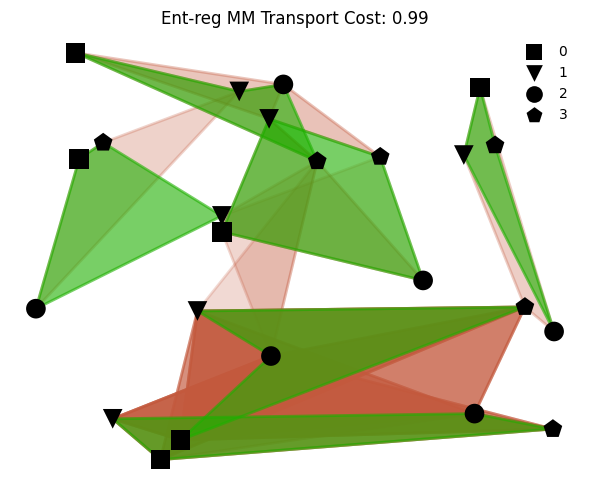
We can now plot some elements of the multimarginal OT tensor, by representing 4-tuples as polygons.

Because the marginal distributions are uniform, and the number of points in each point cloud is the same (here 6), we expect that the OT tensor will be close, numerically, to a polymatching tensor of size \(6^4\).

We list top_k = 24 4-tuples, namely those that have the largest transport values. Each is displayed as a quadrilateral linking those 4 points. The top \(n\) are displayed in green, depicting the most probable mapping, next we color the quadrilaterals in red at an alpha transparency value that is proportional to the transported mass (the darker, the more mass).

cmap = colors.ListedColormap(["#1eb000", "#c3593d"])
top_k = 24


def plot_clouds(
    out: mmsinkhorn.MMSinkhornOutput,
    top_k: Optional[int] = None,
) -> None:
    fig, ax = plt.subplots(figsize=(6, 5), tight_layout=True)
    plott = plot.PlotMM(fig=fig, ax=ax, cmap=cmap)
    _ = plott(out, top_k=top_k)

    ax.set_title(f"Ent-reg MM Transport Cost: {out.ent_reg_cost:.2f}")
    ax.legend(frameon=False, markerscale=0.85)
    ax.axis("off")


plot_clouds(out, top_k=top_k)

Stability of entropy-regularized Multimarginal OT

The analogy to Sinkhorn in the multi-marginal case, looking only for a single polygon between points, is a fairly complicated linear program that was studied recently and shown to be not reducible to a network flow problem [Lin et al., 2022]. The algorithm is extremely slow (\(n^{3k}\)), Whereas the multimarginal Sinkhorn is \(n^{k}\), it is still a fairly heavy price tag, but it’s much easier to implement and differentiate through.

Here we compare the dynamics of mappings when considering the entropy-regularized solution, providing weights to all polygons, vs. selecting a single polygon per data point while perturbing one measure.

def display_animation(
    ots: list[mmsinkhorn.MMSinkhornOutput],
    top_k: Optional[int] = None,
    titles: Optional[list[str]] = None,
    frame_rate: int = 5,
) -> None:
    fig = plt.figure(figsize=(6, 5))
    plott = plot.PlotMM(fig=fig, cmap=cmap)
    anim = plott.animate(ots, top_k=top_k, titles=titles, frame_rate=frame_rate)
    html = display.HTML(anim.to_jshtml())
    display.display(html)
    plt.close()


def random_jitter(
    rng: jax.Array,
    k: int = 4,
    n: int = 6,
    frames: int = 100,
    epsilon: float = 1e-2,
) -> list[mmsinkhorn.MMSinkhornOutput]:
    solver = jax.jit(mmsinkhorn.MMSinkhorn())
    n_s, d = [n] * k, 2

    rng, rng0 = jax.random.split(rng, 2)
    rngs = jax.random.split(rng, k)
    rngs0 = jax.random.split(rng0, k)
    x_s = [jax.random.uniform(rng, (n, d)) for rng, n in zip(rngs, n_s)]
    x_s0 = [jax.random.uniform(rng, (n, d)) for rng, n in zip(rngs0, n_s)]

    ots = []
    for t in jnp.linspace(0, 1, frames):
        x_c = x_s.copy()
        for i in range(k):
            x_c[i] = (
                jnp.clip(((1 - t) * x_s[i] + t * x_s0[i]), 0, 1)
                if i == 0
                else x_c[i]
            )
        ot = solver(x_c, epsilon=epsilon)
        ots.append(ot)

    return ots

# compute and display the stability of regularized MM-OT cost.
ots = random_jitter(jax.random.PRNGKey(0), k=k, n=n)
titles = [f"Iter {i}: Ent-Reg MM OT Mapping" for i in range(len(ots))]
display_animation(ots, top_k=top_k, titles=titles)

Once Loop Reflect

# compare the `Ent-reg  MM-OT` dynamics to the dynamics when considering only the optimal (maximal) matching, a.k.a ignoring weights.
titles = [f"Iter {i}: Ent-reg MM Mapping" for i in range(len(ots))]
display_animation(ots, titles=titles)

Once Loop Reflect

As the MM-OT solution highlights the polygons between all points, rather than the limited set of optimal matches, it is differentiable, and we can look into the gradient flows induced by differentiating the solution.

Gradient Flow

Suppose the points in x_s[0] stay fixed, and that all other 3 point clouds can be moved. To decrease their entropy-regularized MM transport cost, we can use gradient descent. Here, the MMSinkhorn solver uses by default the [Danskin, 1967] theorem to facilitate the computation of the gradient of the entropy regularized cost w.r.t. the point cloud locations.

def objective(
    x_s: list[jnp.ndarray],
    a_s: Optional[list[jnp.ndarray]] = None,
    epsilon: float = 1e-2,
) -> tuple[float, mmsinkhorn.MMSinkhornOutput]:
    out = mmsinkhorn.MMSinkhorn()(x_s=x_s, a_s=a_s, epsilon=epsilon)
    return out.ent_reg_cost, out


def gradient_flow(
    rng: jax.Array,
    k: int = 4,
    n: int = 6,
    n_iters: int = 100,
    epsilon: float = 1e-2,
    lr: float = 0.05,
) -> list[mmsinkhorn.MMSinkhornOutput]:
    n_s, d = [n] * k, 2
    objective_v_g = jax.jit(jax.value_and_grad(objective, has_aux=True))

    rngs = jax.random.split(rng, k)
    x_s = [jax.random.uniform(rng, (n, d)) for rng, n in zip(rngs, n_s)]

    ots = []
    for _ in range(n_iters):
        (v, ot), g_s = objective_v_g(x_s, a_s=None, epsilon=epsilon)
        x_s = [x_s[0]] + [x - lr * g for x, g in zip(x_s[1:], g_s[1:])]
        ots.append(ot)

    return ots

Notice that the entropy regularized cost decreases, and becomes even negative. This is not unusual, since unlike the standard MM-OT cost which is necessarily non-negative, this output is regularized with a negative entropy.

ots = gradient_flow(jax.random.PRNGKey(0), k=k, n=n)
titles = [
    f"Iter {i}: Ent-reg MM Transport Cost: {ot.ent_reg_cost:.2f}"
    for i, ot in enumerate(ots)
]
display_animation(ots, top_k=top_k, titles=titles)

Once Loop Reflect