Sharded Sinkhorn

# Misc.
import functools
import time
from typing import Optional

# Jax and sharding utils
import jax
import jax.numpy as jnp
from jax.experimental import mesh_utils

import matplotlib.pyplot as plt

# Ott
from ott.data import get_cifar10
from ott.geometry import costs, pointcloud
from ott.math import utils
from ott.solvers import linear
from ott.solvers.linear import sinkhorn

We show in this notebook how calls the Sinkhorn solver can be scaled to handle a hundred thousand points (and possibly more) in dimension 3k using data sharding across multiple GPUs. We start by loading the CIFAR-10 train fold, originally of size 50k, duplicated using horizontal flips.

x, y, label = get_cifar10(
    sigma=1.0, gaussian_blur_kernel_size=15, use_flip=True
)

This loads two point-clouds in dimension 3072 of 100k points each.

x.shape, y.shape

((100000, 3072), (100000, 3072))

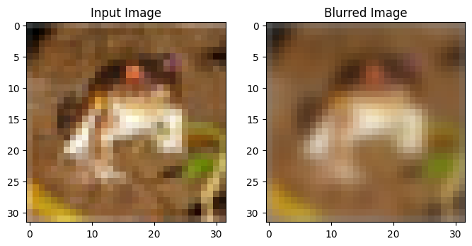
The source x contains all images. The target y contains the same images, to which a Gaussian blur has been applied. This blurring operation is an optimal transport: as shown in [Kassraie et al., 2024], an optimal transport solver parameterized with a squared-Euclidean cost should match x to y exactly in that order. In other words, the optimal transport matrix should be the identity divided by 100k, each image is optimally matched to its blurred counterpart.

plt.figure(figsize=(8, 5))
plt.subplot(1, 2, 1)
plt.imshow(x[0].reshape((3, 32, 32)).transpose(1, 2, 0) / 2 + 0.5)
plt.title("Input Image")
plt.subplot(1, 2, 2)
plt.title("Blurred Image")
plt.imshow(y[0].reshape((3, 32, 32)).transpose(1, 2, 0) / 2 + 0.5)
plt.show()

We run this notebook on a node of 8 GPUs (A100), as is revealed in this call.

jax.devices()

[CudaDevice(id=0),
 CudaDevice(id=1),
 CudaDevice(id=2),
 CudaDevice(id=3),
 CudaDevice(id=4),
 CudaDevice(id=5),
 CudaDevice(id=6),
 CudaDevice(id=7)]

We introduce a simple convenience wrapper designed to shard the input point clouds x and y across 8 GPUs. A more advanced sharding across multiple nodes can be carried out if necessary.

from jax.sharding import Mesh, NamedSharding
from jax.sharding import PartitionSpec as P


def shard_samples(x: jnp.ndarray) -> tuple[jnp.ndarray, NamedSharding]:
    num_devices = jax.device_count()
    devices = mesh_utils.create_device_mesh((num_devices,))
    mesh = Mesh(devices, axis_names=("batch",))
    sharding = NamedSharding(mesh, P("batch", None))

    return jax.device_put(x, sharding), sharding

The inputs are both sharded, and we store that sharding information.

x_sharded, _ = shard_samples(x)
y_sharded, sharding = shard_samples(y)

The run function is a wrapper around a Sinkhorn solver. The batch_size parameter is unchanged, and set to None by default. This means that the full 100k x 100k cost matrix will be materialized, and stored in blocks across multiple GPUs. If that batch_size argument is set to an integer, the cost matrix would be re-instantiated at each iteration, using blocks of 100k x batch_size. Although the code below would still be able to run in the default setting, we advocate using a large batch size in practice.

Note that we use the NegDotProduct cost function to obtain better efficiency, as outlined in [Zhang et al., 2025].

# x, y, epsilon
in_shardings = (sharding, sharding, None)


@functools.partial(
    jax.jit, static_argnames=("batch_size",), in_shardings=in_shardings
)
def run(
    x: jnp.ndarray,
    y: jnp.ndarray,
    epsilon: Optional[float] = None,
    batch_size: Optional[int] = None,
) -> sinkhorn.SinkhornOutput:
    geom = pointcloud.PointCloud(
        x,
        y,
        cost_fn=costs.NegDotProduct(),
        batch_size=batch_size,
        epsilon=epsilon,
        relative_epsilon="std",  # Epsilon is passed as a multiplier for the std of the cost matrix.
    )
    return linear.solve(geom)

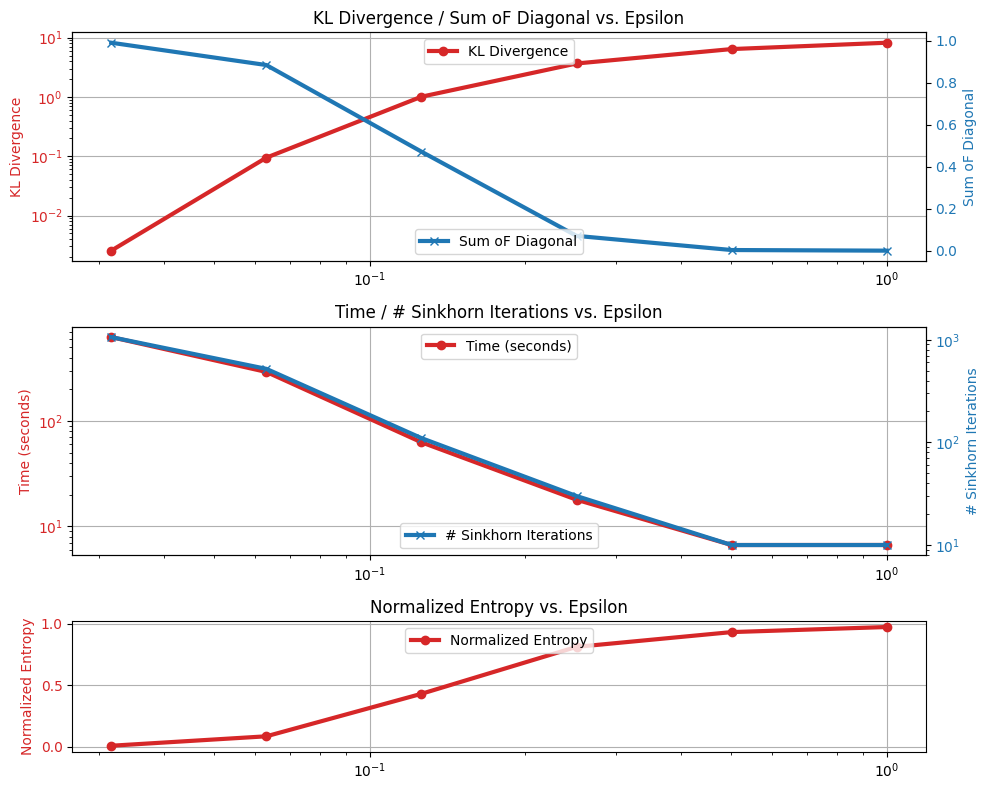
Since the expected optimal coupling should be I_n/n, we simply compute to what extent the output of the Sinkhorn algorithm resembles that matrix. We extract its diagonal and compute its sum (should be close to 1 when using a small epsilon), or alternatively its generalized KL to 1_n/n. We carry out that computation over a grid of 10 epsilon values.

n = x.shape[0]
kls = []
sums = []
times = []
norm_ents = []
num_iters = []
epsilons = 10 ** jnp.linspace(-1.5, 0, 6)
# Run the Sinkhorn solver with different epsilon values
for epsilon in epsilons:
    start = time.time()
    out = run(x_sharded, y_sharded, epsilon, 25_000)
    assert (
        out.converged
    ), f"Sinkhorn did not converge in {out.n_iters} iterations"
    times.append(time.time() - start)
    diag = out.diag
    kls.append(utils.gen_kl(jnp.ones((n,)) / n, diag))
    sums.append(jnp.sum(diag))
    num_iters.append(out.n_iters)
    norm_ents.append(out.normalized_entropy)

These results are summarized in plots below, displaying also running time, number of iterations and normalized entropy (as presented as a function of epsilon.

plt.figure(figsize=(10, 8))
ax_met = plt.subplot2grid((8, 1), (0, 0), rowspan=3)
ax_times = plt.subplot2grid((8, 1), (3, 0), rowspan=3)
ax_norment = plt.subplot2grid((8, 1), (6, 0), rowspan=2)


def plot_two_y(ax, x, y1, y2, label1, label2, log1, log2, title):
    color = "tab:red"
    ax.plot(x, y1, color=color, marker="o", linewidth=3, label=label1)
    ax.set_ylabel(label1, color=color)
    ax.tick_params(axis="y", labelcolor=color)
    ax.set_xscale("log")
    if log1:
        ax.set_yscale("log")
    ax.set_title(title)
    ax.legend(loc="upper center")
    ax.grid(True)

    if y2 is not None:
        color = "tab:blue"
        ax2 = ax.twinx()
        ax2.set_ylabel(label2, color=color)
        ax2.plot(
            epsilons, y2, color=color, marker="x", linewidth=3, label=label2
        )
        ax2.legend(loc="lower center")
        ax2.tick_params(axis="y", labelcolor=color)
        if log2:
            ax2.set_yscale("log")


plot_two_y(
    ax_met,
    epsilons,
    kls,
    sums,
    "KL Divergence",
    "Sum oF Diagonal",
    True,
    False,
    "KL Divergence / Sum oF Diagonal vs. Epsilon",
)
plot_two_y(
    ax_times,
    epsilons,
    times,
    num_iters,
    "Time (seconds)",
    "# Sinkhorn Iterations",
    True,
    True,
    "Time / # Sinkhorn Iterations vs. Epsilon",
)
plot_two_y(
    ax_norment,
    epsilons,
    norm_ents,
    None,
    "Normalized Entropy",
    None,
    False,
    True,
    "Normalized Entropy vs. Epsilon",
)

plt.tight_layout()