Wasserstein Barycenter

import jax
import jax.numpy as jnp

import matplotlib.pyplot as plt

from ott.problems.linear import barycenter_problem
from ott.solvers.linear import continuous_barycenter, sinkhorn

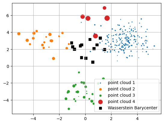
We illustrate in this notebook how to use the FreeWassersteinBarycenter solver to compute the Wasserstein barycenter of either one or multiple probability distributions. We start by generating a few 2D point clouds of varying support size.

ns = (193, 20, 27, 5)  # number of points per cloud
offsets = (
    jnp.array((3.0, 3.0)),
    jnp.array((-3.0, 3.0)),
    jnp.array((0.0, -3.0)),
    jnp.array((0.0, 5.0)),
)  # offsets for each cloud
d = 2  # dimension of the points
k = 13  # number of points in the barycenter's support

keys = jax.random.split(jax.random.key(0), 4)

point_clouds = []
weights = []

for key, n, offset in zip(keys, ns, offsets):
    k1, k2 = jax.random.split(key)
    point_clouds.append(jax.random.normal(k1, (n, d)) + offset)
    weight = jax.random.uniform(k2, (n,))
    weight /= weight.sum()
    weights.append(weight)

flattened_points = jnp.concatenate(point_clouds, axis=0)
flattened_weights = jnp.concatenate(weights, axis=0)

A Wasserstein barycenter problem is defined by a list of (weighted) points clouds (here passed as a flattened array, providing boundaries in num_per_segment) and an epsilon regularization (here set automatically following a scaling rule, since we pass None).

bprob = barycenter_problem.FreeBarycenterProblem(
    y=flattened_points, b=flattened_weights, num_per_segment=ns, epsilon=None
)

Next, we instantiate the solver that will be used to compute the barycenter. We rely on default parameters for number of iterations / tolerance, but we must set the linear solver used within the inner loop iterations, here the Sinkhorn algorithm.

solver = continuous_barycenter.FreeWassersteinBarycenter(
    linear_solver=sinkhorn.Sinkhorn()
)

We jit the solver first and apply it to the problem above.

jitted_solver = jax.jit(solver, static_argnames="bar_size")
out = jitted_solver(bprob, bar_size=k)

The out object contains relevant information about the barycenter itself, notably its points and how the cost evolved throughout iterations

print("Shape of barycenter : ", out.x.shape)
print(
    "Convergence of inner loop iterations :", out.all_linear_solvers_converged
)
print("Converged in:", out.num_iters, "outer iterations.")
print("Objective: ", out.costs_along_iterations)

Shape of barycenter :  (13, 2)
Convergence of inner loop iterations : True
Converged in: 5 outer iterations.
Objective:  [23.27366  15.290319 15.27664  15.271326 15.267798]

Visualize results

base_size = 500
for i, (weight, point_cloud) in enumerate(zip(weights, point_clouds)):
    plt.scatter(
        point_cloud[:, 0],
        point_cloud[:, 1],
        s=base_size * weight,
        label="point cloud " + str(i + 1),
    )
plt.scatter(
    out.x[:, 0],
    out.x[:, 1],
    s=base_size * out.a,
    c="black",
    marker="s",
    label="Wasserstein Barycenter",
)
plt.legend()
plt.grid(True)
plt.show()

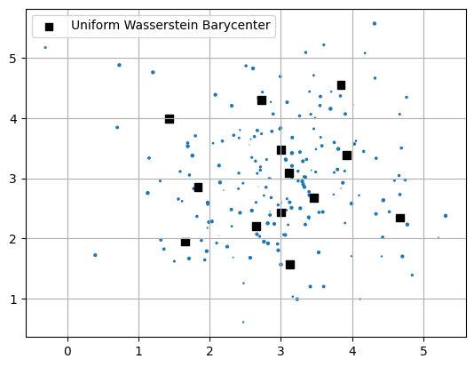
Note that the Wasserstein barycenter problem can also be instantiated on a single measure, to generate a uniformly weighted variant of the \(k\)-means algorithm as described in [Cuturi and Doucet, 2014]. This can be done trivially by describing a problem with a single measure.

bprob = barycenter_problem.FreeBarycenterProblem(
    y=point_clouds[0], b=weights[0], num_per_segment=(ns[0],)
)
out = jitted_solver(bprob, bar_size=k)

When displaying the barycenter, one notices that it is realized by a measure with a smaller support, all points being uniformly weighted.

plt.scatter(
    point_clouds[0][:, 0],
    point_clouds[0][:, 1],
    s=base_size * weights[0],
)
plt.scatter(
    out.x[:, 0],
    out.x[:, 1],
    s=base_size * out.a,
    c="black",
    marker="s",
    label="Uniform Wasserstein Barycenter",
)
plt.legend()
plt.grid(True)
plt.show()