Semidiscrete OT

We show in this notebook how to use OTT to solve a particular type of optimal transport, the semidiscrete problem, in which one wishes to map a continuous distribution to a predefined finite point cloud target.

import jax
import jax.numpy as jnp
import jax.random as jr

import optax

import matplotlib.pyplot as plt

from ott.geometry import costs
from ott.geometry import semidiscrete_pointcloud as sdpc
from ott.problems.linear import semidiscrete_linear_problem as sdlp
from ott.solvers import linear
from ott.solvers.linear import semidiscrete
from ott.tools import plot

Problem definition

We create a SemidiscretePointCloud using:

• the source distribution from which we can sample. The function needs to accept:

  • rng - random number generator,

  • shape - shape of the samples to generate,

  • dtype - the data type of the generated samples,

• the discrete target distribution, an array of shape [m, ...],

• epsilon regularization \(\varepsilon\geq 0\) strength,

• the cost function of type CostFn.

In this tutorial, we use jax.random.normal() as our source distribution and \(\varepsilon=0\), which corresponds to the unregularized semidiscrete problem, and pick a fixed set of target points in a thick half circle

rng = jr.key(0)
rng_data, rng_solve, rng_sample_geom, rng_sample_out = jr.split(rng, 4)

# Plot target points in (roughly) half circle
m, d = 96, 2
rng1, rng2 = jr.split(rng_data)
y = jr.normal(rng1, (m, d))
y /= jnp.linalg.norm(y, axis=-1, keepdims=True)  # sphere
y *= 2 * jr.uniform(rng2, (m,))[:, None] + 3
y = y.at[:, 0].set(jnp.abs(y[:, 0]))

geom = sdpc.SemidiscretePointCloud(
    sampler=jr.normal,
    y=y,
    epsilon=0.0,
    cost_fn=costs.SqEuclidean(),
)

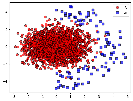
We can now sample from the source distribution and create a PointCloud instance using the sample() method.

sampled_geom = geom.sample(rng_sample_geom, 2048)  # sample 256 points

fig, ax = plt.subplots()
dict_kw = plot.get_plotkwargs(background=False)

x = sampled_geom.x
ax.scatter(x[:, 0], x[:, 1], **dict_kw["x"])
ax.scatter(sampled_geom.y[:, 0], sampled_geom.y[:, 1], **dict_kw["y"])
_ = ax.legend()

Solving the semidiscrete OT problem

We can solve the (unregularized) semidiscrete problem using the SemidiscreteSolver. Important arguments to the solver include:

• num_iterations - total number of iterations,

• batch_size - number of samples to draw from the source distribution at each iteration,

• optimizer - optimizer to use, such as optax.sgd().

error_eval_every = 5000


def print_callback(state: semidiscrete.SemidiscreteState) -> None:
    it = state.it.item()
    if it > 0 and it % error_eval_every == 0:
        loss = state.errors[it // error_eval_every - 1].item()
        print(f"It. {it:5d}, marginal χ2 error={loss:.4f}")


@jax.jit
def solve_semidiscrete(
    rng: jax.Array, geom: sdpc.SemidiscretePointCloud
) -> semidiscrete.SemidiscreteOutput:
    prob = sdlp.SemidiscreteLinearProblem(geom)
    solver = semidiscrete.SemidiscreteSolver(
        num_iterations=40_000,
        batch_size=128,
        optimizer=optax.sgd(learning_rate=0.02),
        error_eval_every=error_eval_every,
        callback=print_callback,
    )
    return solver(rng, prob)

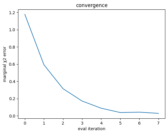
We evaluate and print the marginal χ2 error between the ground-truth and estimated target marginal every 5000 iterations.

out = solve_semidiscrete(rng, geom)

It.  5000, marginal χ2 error=1.1769
It. 10000, marginal χ2 error=0.5923
It. 15000, marginal χ2 error=0.3147
It. 20000, marginal χ2 error=0.1715
It. 25000, marginal χ2 error=0.0881
It. 30000, marginal χ2 error=0.0379
It. 35000, marginal χ2 error=0.0423
It. 40000, marginal χ2 error=0.0283

And plot the evolution of the marginal χ2 error along the iterations.

fig, ax = plt.subplots()
ax.plot(out.errors)
ax.set_title("convergence")
ax.set_xlabel("eval iteration")
_ = ax.set_ylabel("marginal χ2 error")

We can use SemidiscreteOutput.sample to sample some points from the from the source distribution and compute the optimal transport plan between these points and the target distribution.

In the unregularized case \(\varepsilon = 0\), the transport matrix will be stored as a sparse BCOO matrix.

out_sampled = out.sample(rng_sample_out, 16)
out_sampled.matrix

BCOO(float32[16, 96], nse=16)

_, col_ixs = out_sampled.matrix.indices.T

sampled_geom = out_sampled.ot_prob.geom
x_new = sampled_geom.x
y_new = sampled_geom.y
matched_y = y[col_ixs]
delta = matched_y - x_new

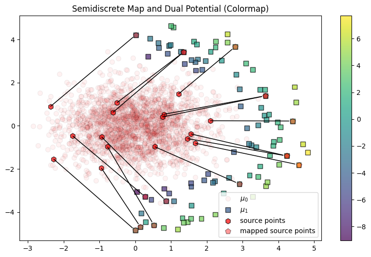
Below, we show the sampled source points along with their matches in the target distribution. Notice how two different source points can be matched to the same target point, which is obviously bound to happen since an infinite set of points must land on the finite target for the map to be valid.

fig, ax = plt.subplots(figsize=(10, 6))
# A few changes to plot defaults
dict_kw["x"].update({"alpha": 0.05})  # let source points fade
dict_kw["y"].pop("color", None)  # remove original color
dict_kw["y"].update({"c": out.g})  # plot dual variables on top
dict_kw["txnew"].update({"alpha": 0.4})  # transparency to show overloap with y

ax.scatter(x[:, 0], x[:, 1], **dict_kw["x"])
bar = ax.scatter(y[:, 0], y[:, 1], **dict_kw["y"])

ax.scatter(x_new[:, 0], x_new[:, 1], **dict_kw["xnew"], label="source points")
ax.scatter(
    matched_y[:, 0],
    matched_y[:, 1],
    **dict_kw["txnew"],
    label="mapped source points",
)

ax.quiver(
    x_new[:, 0],
    x_new[:, 1],
    delta[:, 0],
    delta[:, 1],
    scale_units="xy",
    angles="xy",
    scale=1.0,
    width=0.0025,
    headwidth=0,
)
fig.colorbar(bar)
plt.title("Semidiscrete Map and Dual Potential (Colormap)")
_ = ax.legend(loc="best")